6. Gene and variant annotations
After this chapter, the students can explain the concepts “gene annotation” and “variant annotation” and their roles in analyses of population genetic data. They can evaluate the pitfalls of different automated prediction approaches and choose a suitable method for their own data.
Neutral and non-neutral sites
Early population genetics built on Charles Darwin’s work and natural selection had a central role. Given the omnipresent selection, the appearance of genetic variation and alternative alleles had to be explained by balancing selection and other active forces. The neutral theory by Motoo Kimura challenged that and proposed that much of the genetic variation is neutral and the changes are driven by random processes. This started a long-lasting war between selectionists and neutralists.
The Wright-Fisher population model and the coalescence model assume that the sites studied are neutral and the changes in allele frequencies are a result of a stochastic process and not affected by selection. Many of the analyses on this course are based on this assumption. The assumption of neutrality doesn’t necessarily need to be strict: can assume that a majority of sites are evolving roughly neutrally and the sites under strong directional selection are rare enough not to significantly affect the analyses.
Although we have assumed “rough neutrality”, we have not specifically defined what makes the process “neutral” and how we know that the sites are evolving “neutrally”. One reason for the omissions it that showing specific sites to evolve neutrally is difficult. Showing that specific sites evolve non-neutrally is slightly easier, and predicting that certain sites probably do not evolve neutrally is even easier.
The easiest criterion to predict that site is under selection (and not evolving neutrally) is to show that it has a biological function based on the DNA sequence; many (but not necessarily all) changes in the DNA sequence break this biological function and affect the fitness of the individual carrying the mutation, thus triggering selection on the mutation.
What is then a biological function? The Encyclopedia Of DNA Elements (ENCODE) was a major undertaking to understand the human genome. One of the controversial claims of the final publication (ref and ref) was that 80% of the human genome has a biochemical function. This claim was trashed by evolutionary biologists (ref, ref and ref). There is little progress since then and it is still unclear what is a real “function” and when an “effect” is mere noise.
Gene annotation
Although we mostly assume neutral evolution on this course, sometimes the function is of interest, even the main target of the study. One of the easiest genomic functions to predict is the location of genes, although even there the boundary between the “classical” protein-coding genes and the “new” non-coding genes, i.e.genome regions expressed in a gene-like manner, is getting complicated.
The locations of genes can be predicted in many ways. Protein-coding genes must have open reading frames (ORFs) and, if multi-exonic, proper splice sites. These patterns can be detected computationally, but the resulting predictions are rough and noisy. In practice, de novo inference is done from biological data, the spliced transcripts (or peptides) generated by the organisms. Messenger RNAs (mRNAs) can be extracted and sequenced similarly to the genome’s DNA sequence; these sequencing reads can then be mapped to the genome, taking into account the exon structure. A downside of this approach is that all genes are not expressed everywhere, all the time and in equal quantities. This is tackled by combining data from multiple tissues (in a case of an animal, e.g. muscle, liver, testis, brain) and increasing the sequencing depth.
Even with good resources, it is extremely difficult (or impossible) to cover all genes and alternative transcripts of a complex organism. Furthermore, the transcriptome of a species is not fixed: in addition to allelic differences within genes, there are differences in gene presence/absence and gene copy number between populations and individuals.
In A beginner’s guide to eukaryotic genome annotation, the authors write:
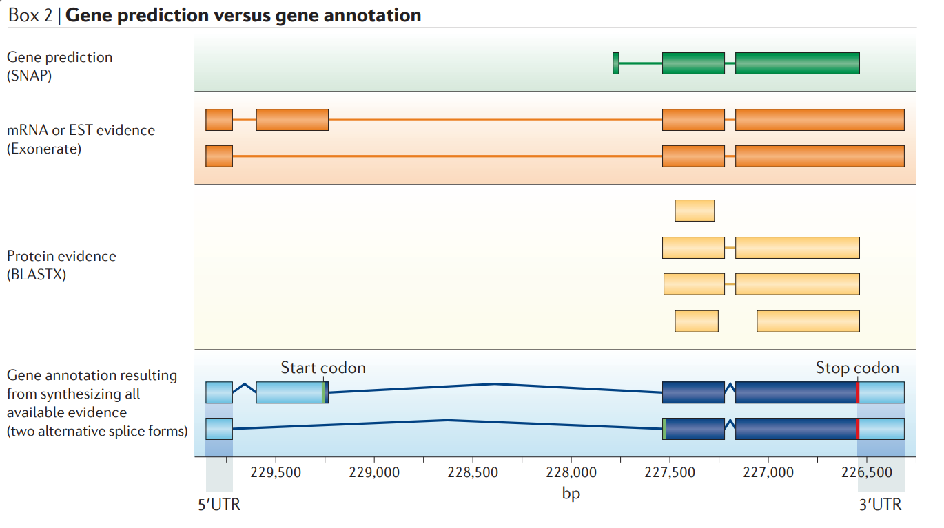
Although the terms ‘gene prediction’ and ‘gene annotation’ are often used as if they are synonyms, they are not. With a few exceptions, gene predictors find the single most likely coding sequence (CDS) of a gene and do not report untranslated regions (UTRs) or alternatively spliced variants. Gene prediction is therefore a somewhat misleading term. A more accurate description might be ‘canonical CDS prediction’.
Gene annotations, conversely, generally include UTRs, alternative splice isoforms and have attributes such as evidence trails. The figure shows a genome annotation and its associated evidence. Terms in parentheses are the names of commonly used software tools for assembling particular types of evidence. Note that the gene annotation (shown in blue) captures both alternatively spliced forms and the 5′ and 3′UTRs suggested by the evidence. By contrast, the gene prediction that is generated by SNAP (shown in green) is incorrect as regards the gene’s 5′ exons and start-of-translation site and, like most gene-predictors, it predicts only a single transcript with no UTR.
Gene annotation is thus a more complex task than gene prediction. A pipeline for genome annotation must not only deal with heterogeneous types of evidence in the form of the expressed sequence tags (ESTs), RNA-seq data, protein homologies and gene predictions, but it must also synthesize all of these data into coherent gene models and produce an output that describes its results in sufficient detail for these outputs to become suitable inputs to genome browsers and annotation databases.
On this course, we do not do de novo gene prediction but use homology and transfer the gene predictions from another species, the three-spined stickleback that is included in the major genome databases.
Structure of a gene
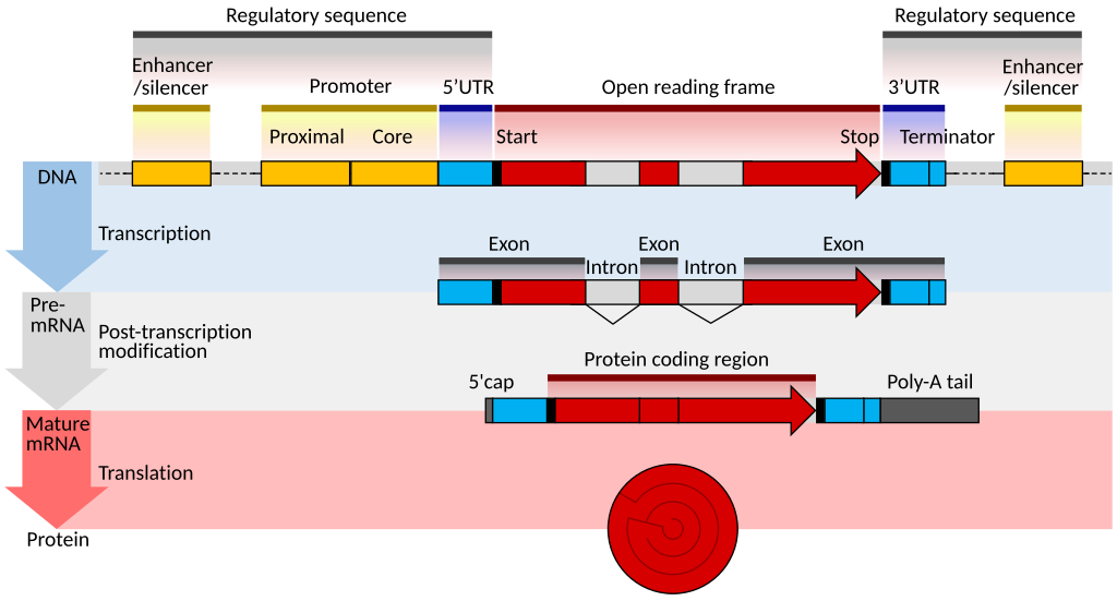
The gene structure is described in the Wikipedia article like this:
In the upper-most row, the different elements are indicated with different colours and, in principle, our genome annotation could include all of these. In practice, the gene annotation often consists of the red blocks only. The grey blocks, introns’ can then be defined, as well as proximity to a gene, e.g. “upstream of gene” (sometimes called “promoter”), “downstream of gene” etc.
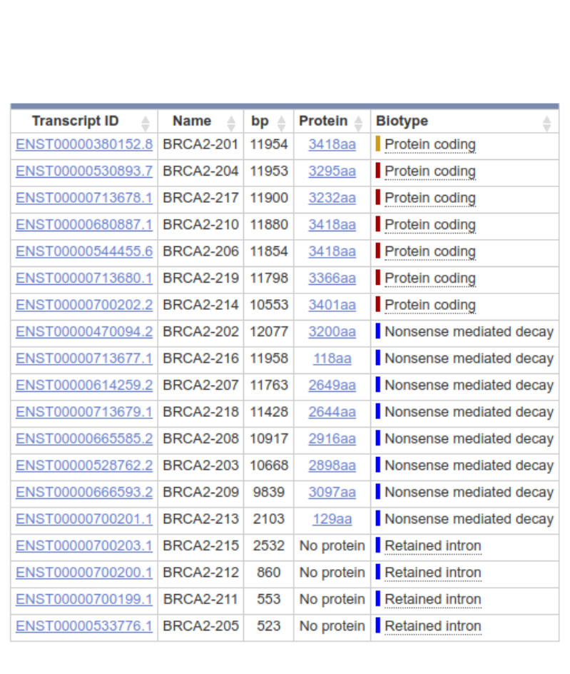
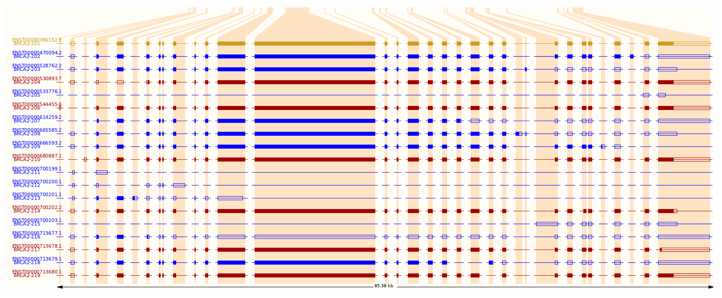
This figure lacks details, however, and especially in more complex organisms, genes often produce multiple different transcripts, some of which may be non-functional and directed immediately to a decay pathway. The figures below show the alternative transcripts of the human BRCA2 gene:
Such accurate annotations are not available for many other species.
Annotation lift-over
There are different ways of transferring the information from a closely-related model species to the target species. People behind the UCSC genome browser developed a tool called LifOver to convert coordinates in one genome to those in another genome, and called this transfer “lifting”. If one has a description of homologous regions in the two genomes, the procedure is pretty simple. Let’s assume that a region in ctg2078 in species_A would be homologous to a region in chr3 in species_B. We could then write conversion tables like these to convert a coordinate in one species to another:
ctg2078 19679   chr3    207555
ctg2078 19680   chr3    207556
ctg2078 19681   chr3    207557
ctg2078 19682   chr3    207558
ctg2078 19683   chr3    207559
ctg2078 19684   chr3    207560
ctg2078 19685   chr3    207561
ctg2078 19686   chr3    207562
ctg2078 19687   chr3    207563
ctg2078 19688   chr3    207564
ctg2078 19689   chr3    207566
ctg2078 19690   chr3    207567
ctg2078 19691   chr3    207568
ctg2078 19692   chr3    207569
ctg2078 19693   chr3    207570
ctg2078 19694   chr3    207571
ctg2078 19695   chr3    207572
From species_A (cols 1,2) to species_B (cols 3,4)
chr3    207555  ctg2078 19679
chr3    207556  ctg2078 19680
chr3    207557  ctg2078 19681
chr3    207558  ctg2078 19682
chr3    207559  ctg2078 19683
chr3    207560  ctg2078 19684
chr3    207561  ctg2078 19685
chr3    207562  ctg2078 19686
chr3    207563  ctg2078 19687
chr3    207564  ctg2078 19688
chr3    207565  NA      NA
chr3    207566  ctg2078 19689
chr3    207567  ctg2078 19690
chr3    207568  ctg2078 19691
chr3    207569  ctg2078 19692
chr3    207570  ctg2078 19693
chr3    207571  ctg2078 19694
chr3    207572  ctg2078 19695
From species_B (cols 1,2) to species_A (cols 3,4)
To convert “ctg2078:19685” to “chr3:207561”, we would just need to find a row where the first two columns match and then read the new coordinate in the last two columns. To do it other way round, the position of columns are swapped (right).
Space-wise, this would be very inefficient, however. We can see that most sites follow in order and there is only one small gap in the other genome. If the genome would large, this kind of an index file would be several gigabytes in size and very slow to read into computer memory.
The same task is done in a more compact way by using the Chain Format. The one above is an artificial example, but the same information could be stored e.g. in this manner:
chain 1200 ctg2078 56789 + 19679 19696 chr3 5456798 + 207555 207573
10 0 1
7
(Many numbers above are completely arbitrary.)
There’s a program chainSwap that can swap the direction of the chain:
chain 1200 chr3 5456798 + 207555 207573 ctg2078 56789 + 19679 19696 1
10  1   0
7
In practice, the chains are of course much longer and more complex, but they are very space-efficient.
With a lift-over chain, the positions in one genome can be converted to positions in another genome. Note, though, that some genome regions may be unique to one species, evolved beyond recognition or been duplicated, and all the positions are rarely included in a chain file. If the sites are missing, the coordinates at those sites cannot be transferred.
A downside of this approach is that the positions in the genome are transferred without any check whether the regions defined in the files show any similarity in the two genomes; it is enough that the start and end positions of the elements are inferred to be homologous. Some “lift-over” programs check that the element transferred to a new genome is exactly as long as the original element: this is often unnecessarily strict and e.g. gene regions tolerate indels within exons and can be correct even with length changes.
Alignment of gene or protein sequences only
The generation of a lit-over chain file used to be a bit cumbersome and, as it requires a full genome alignment, computationally heavy. LifOff provides an alternative approach and only needs to align the regions that are lifted. LiftOff uses the gene annotation for species_A to extract the gene sequences from the species_A’s genome, and then aligns these gene sequences to species_B’s genome. From the resulting alignments, it computes the location of the genes and their exons in species_B’s genome and outputs the information in the structured format of gene annotation.
A variant of this approach is not to use DNA (gene) sequences but protein sequences. There are a few programs that can align protein sequences to genomic sequences, considering the alternative reading frames and exon splicing in the process. The most efficient of these methods is miniprot. The program can output the alignments in a structured format but unfortunately, this format is not directly compatible with all downstream processing tools.
Using the gene structure figure, LiftOff takes the middle row from one species as input and aligns it to the top row of another species; from the alignment, it then calculates the block boundaries. On the other hand, miniprot takes the bottom row from one species as input and aligns it to the top row of another species; from the alignment, it then resolves the block boundaries.
A potentially serious downside of these approaches is that they can’t be used to transfer the locations of small elements, e.g. transcription factor binding sites, from one genome to another: to get reliable alignments, the elements have to be unique and long enough and, in the cases of miniprot, protein-coding.
Variant annotation
Types of consequences
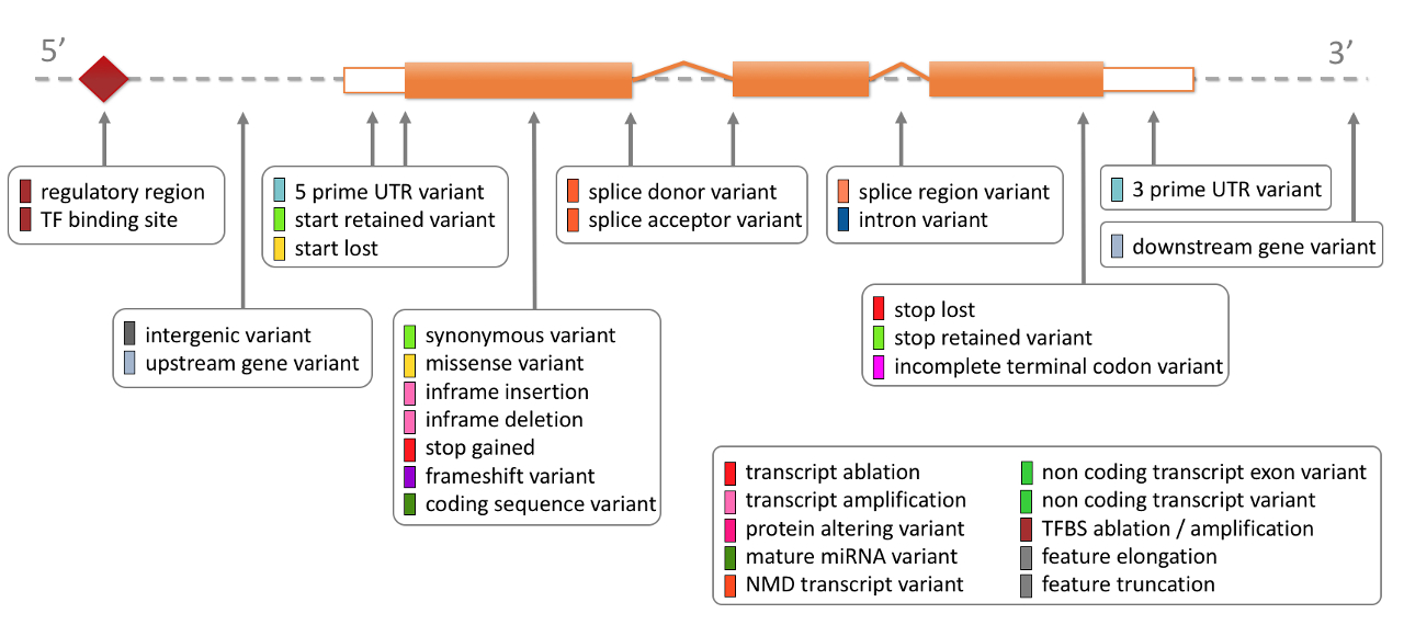
Given the annotation of genes, the location of VCF variants relative to that can be easily solved. Ensembl provides a comprehensive description of the variants contained in their Variation database, visualised below and listed in detail their calculated variant consequences:
The terms in the figure are listed in the table below, shown in order of severity (more severe to less severe) as estimated by Ensembl.
| SO term | SO description | Display term | IMPACT |
|---|---|---|---|
| transcript_ablation | A feature ablation whereby the deleted region includes a transcript feature | Transcript ablation | HIGH |
| splice_acceptor_variant | A splice variant that changes the 2 base region at the 3’ end of an intron | Splice acceptor variant | HIGH |
| splice_donor_variant | A splice variant that changes the 2 base region at the 5’ end of an intron | Splice donor variant | HIGH |
| stop_gained | A sequence variant whereby at least one base of a codon is changed, resulting in a premature stop codon, leading to a shortened transcript | Stop gained | HIGH |
| frameshift_variant | A sequence variant which causes a disruption of the translational reading frame, because the number of nucleotides inserted or deleted is not a multiple of three | Frameshift variant | HIGH |
| stop_lost | A sequence variant where at least one base of the terminator codon (stop) is changed, resulting in an elongated transcript | Stop lost | HIGH |
| start_lost | A codon variant that changes at least one base of the canonical start codon | Start lost | HIGH |
| transcript_amplification | A feature amplification of a region containing a transcript | Transcript amplification | HIGH |
| feature_elongation | A sequence variant that causes the extension of a genomic feature, with regard to the reference sequence | Feature elongation | HIGH |
| feature_truncation | A sequence variant that causes the reduction of a genomic feature, with regard to the reference sequence | Feature truncation | HIGH |
| inframe_insertion | An inframe non synonymous variant that inserts bases into in the coding sequence | Inframe insertion | MODERATE |
| inframe_deletion | An inframe non synonymous variant that deletes bases from the coding sequence | Inframe deletion | MODERATE |
| missense_variant | A sequence variant, that changes one or more bases, resulting in a different amino acid sequence but where the length is preserved | Missense variant | MODERATE |
| protein_altering_variant | A sequence_variant which is predicted to change the protein encoded in the coding sequence | Protein altering variant | MODERATE |
| splice_donor_5th_base_variant | A sequence variant that causes a change at the 5th base pair after the start of the intron in the orientation of the transcript | Splice donor 5th base variant | LOW |
| splice_region_variant | A sequence variant in which a change has occurred within the region of the splice site, either within 1-3 bases of the exon or 3-8 bases of the intron | Splice region variant | LOW |
| splice_donor_region_variant | A sequence variant that falls in the region between the 3rd and 6th base after splice junction (5’ end of intron) | Splice donor region variant | LOW |
| splice_polypyrimidine_tract_variant | A sequence variant that falls in the polypyrimidine tract at 3’ end of intron between 17 and 3 bases from the end (acceptor -3 to acceptor -17) | Splice polypyrimidine tract variant | LOW |
| incomplete_terminal_codon_variant | A sequence variant where at least one base of the final codon of an incompletely annotated transcript is changed | Incomplete terminal codon variant | LOW |
| start_retained_variant | A sequence variant where at least one base in the start codon is changed, but the start remains | Start retained variant | LOW |
| stop_retained_variant | A sequence variant where at least one base in the terminator codon is changed, but the terminator remains | Stop retained variant | LOW |
| synonymous_variant | A sequence variant where there is no resulting change to the encoded amino acid | Synonymous variant | LOW |
| coding_sequence_variant | A sequence variant that changes the coding sequence | Coding sequence variant | MODIFIER |
| mature_miRNA_variant | A transcript variant located with the sequence of the mature miRNA | Mature miRNA variant | MODIFIER |
| 5_prime_UTR_variant | A UTR variant of the 5’ UTR | 5 prime UTR variant | MODIFIER |
| 3_prime_UTR_variant | A UTR variant of the 3’ UTR | 3 prime UTR variant | MODIFIER |
| non_coding_transcript_exon_variant | A sequence variant that changes non-coding exon sequence in a non-coding transcript | Non coding transcript exon variant | MODIFIER |
| intron_variant | A transcript variant occurring within an intron | Intron variant | MODIFIER |
| NMD_transcript_variant | A variant in a transcript that is the target of NMD | NMD transcript variant | MODIFIER |
| non_coding_transcript_variant | A transcript variant of a non coding RNA gene | Non coding transcript variant | MODIFIER |
| coding_transcript_variant | A transcript variant of a protein coding gene | Coding transcript variant | MODIFIER |
| upstream_gene_variant | A sequence variant located 5’ of a gene | Upstream gene variant | MODIFIER |
| downstream_gene_variant | A sequence variant located 3’ of a gene | Downstream gene variant | MODIFIER |
| TFBS_ablation | A feature ablation whereby the deleted region includes a transcription factor binding site | TFBS ablation | MODIFIER |
| TFBS_amplification | A feature amplification of a region containing a transcription factor binding site | TFBS amplification | MODIFIER |
| TF_binding_site_variant | A sequence variant located within a transcription factor binding site | TF binding site variant | MODIFIER |
| regulatory_region_ablation | A feature ablation whereby the deleted region includes a regulatory region | Regulatory region ablation | MODIFIER |
| regulatory_region_amplification | A feature amplification of a region containing a regulatory region | Regulatory region amplification | MODIFIER |
| regulatory_region_variant | A sequence variant located within a regulatory region | Regulatory region variant | MODIFIER |
| intergenic_variant | A sequence variant located in the intergenic region, between genes | Intergenic variant | MODIFIER |
| sequence_variant | A sequence_variant is a non exact copy of a sequence_feature or genome exhibiting one or more sequence_alteration | Sequence variant | MODIFIER |
Coding changes and genetic codes
Traditionally, much of the interest has focused on coding sequence (CDS) variants and, among those, on synonymous and non-synonymous changes. A significant reason behind that is again their relative simplicity and therefore suitability to mathematical modelling.
Synonymous variants affect CDS but do not change the amino acid that the affected codon codes for. In micro-organisms, the efficiency of gene transcription and translation is often optimised to such extent that even the availability of transfer RNAs for different codons and the efficiency of their incorporation matters. In such cases, synonymous codons may have fitness differences and not be selectively neutral. In higher organisms, synonymous variants, as such, are considered to be approximately neutral; however, the gene region with a variant may have other functions than just protein coding, and a neutral variant may be linked to a nearby variant under selection and thus indirectly affected by selection.
Non-synonymous variants – also called missense variants – change the codon such that the encoded amino acid changes. The amino acids differ greatly in their properties and the severity of the change is typically not reported.
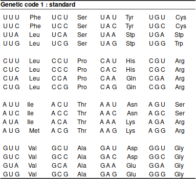
The synonymous and missense mutations are naturally a consequence of the redundancies in the genetic code; several codons code for the same amino acid:
Synonymous changes are mostly in the codon third position but also the codon first position changes can be synonymous. In addition to that, the codon changes caused by first and third position tend to less dramatic than those caused by the second position. As an example of that, we can study the scores in the BLOSUM tables. The series of BLOSUM tables (used e.g. by BLAST) are generated from homologous protein sequences that are diverged for a certain amount. Each amino-acid pair gets a log-odds score that reflects how frequently the pair is observed in the data compared to the changes of seeing them by chance: \[ LogOddRatio = 2 log_2 \left(\frac{P(O)}{P(E)}\right) \]
The scores are highly positive for pairs that are seen frequently, such as Leucine (L) matched with Leucine that has the score 6:
   A  R  N  D  C  Q  E  G  H  I  L  K  M  F  P  S  T  W  Y  V
A  7 -3 -3 -3 -1 -2 -2  0 -3 -3 -3 -1 -2 -4 -1  2  0 -5 -4 -1
R -3  9 -1 -3 -6  1 -1 -4  0 -5 -4  3 -3 -5 -3 -2 -2 -5 -4 -4
N -3 -1  9  2 -5  0 -1 -1  1 -6 -6  0 -4 -6 -4  1  0 -7 -4 -5
D -3 -3  2 10 -7 -1  2 -3 -2 -7 -7 -2 -6 -6 -3 -1 -2 -8 -6 -6
C -1 -6 -5 -7 13 -5 -7 -6 -7 -2 -3 -6 -3 -4 -6 -2 -2 -5 -5 -2
Q -2  1  0 -1 -5  9  3 -4  1 -5 -4  2 -1 -5 -3 -1 -1 -4 -3 -4
E -2 -1 -1  2 -7  3  8 -4  0 -6 -6  1 -4 -6 -2 -1 -2 -6 -5 -4
G  0 -4 -1 -3 -6 -4 -4  9 -4 -7 -7 -3 -5 -6 -5 -1 -3 -6 -6 -6
H -3  0  1 -2 -7  1  0 -4 12 -6 -5 -1 -4 -2 -4 -2 -3 -4  3 -5
I -3 -5 -6 -7 -2 -5 -6 -7 -6  7  2 -5  2 -1 -5 -4 -2 -5 -3  4
L -3 -4 -6 -7 -3 -4 -6 -7 -5  2  6 -4  3  0 -5 -4 -3 -4 -2  1
K -1  3  0 -2 -6  2  1 -3 -1 -5 -4  8 -3 -5 -2 -1 -1 -6 -4 -4
M -2 -3 -4 -6 -3 -1 -4 -5 -4  2  3 -3  9  0 -4 -3 -1 -3 -3  1
F -4 -5 -6 -6 -4 -5 -6 -6 -2 -1  0 -5  0 10 -6 -4 -4  0  4 -2
P -1 -3 -4 -3 -6 -3 -2 -5 -4 -5 -5 -2 -4 -6 12 -2 -3 -7 -6 -4
S  2 -2  1 -1 -2 -1 -1 -1 -2 -4 -4 -1 -3 -4 -2  7  2 -6 -3 -3
T  0 -2  0 -2 -2 -1 -2 -3 -3 -2 -3 -1 -1 -4 -3  2  8 -5 -3  0
W -5 -5 -7 -8 -5 -4 -6 -6 -4 -5 -4 -6 -3  0 -7 -6 -5 16  3 -5
Y -4 -4 -4 -6 -5 -3 -5 -6  3 -3 -2 -4 -3  4 -6 -3 -3  3 11 -3
V -1 -4 -5 -6 -2 -4 -4 -6 -5  4  1 -4  1 -2 -4 -3  0 -5 -3  7
If we have a closer look on the scores for Leucine pairing with any other amino acid, we can see that the biggest scores are for amino acids whose codons differ from Leucine by a codon first position change:
AA          Leu  Met  Ile  Val  Phe  Tyr  Ala  Cys  Thr  Arg  Gln  Lys  Ser  Trp  His  Pro  Asn  Glu  Asp  Gly
score(Leu)  6    3    2    1    0    -2   -3   -3   -3   -4   -4   -4   -4   -4   -5   -5   -6   -6   -7   -7
Those amino acids are also chemically the most similar.
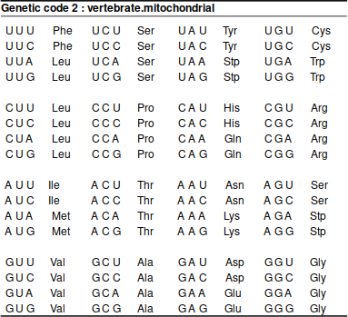
If studying something else but the nuclear DNA of common animals or plants, it is important to consider the genetic code. The most frequently needed alternative code is that for vertebrate mitochondrion:
The difference is not huge but, as the affected codons mostly code for stop codons, highly significant:
          TGA  ATA  AGA  AGG
Standard  *    I    R    R
Vet_Mito  W    M    *    *
The NCBI website list 33 different genetic codes!
Combined effects
When inferring the impact of a variant, it is crucial to note that the nearby variants may jointly have a different consequence than anyone alone. Let’s assume that we have three genomic positions that together form the codon “TAT” and code for Tyrosine, and an individual is heterozygous at the second and third position:
chr    1234    T   .   0/0
chr    1235    A   G   0/1
chr    1236    T   G   0/1
It is now important to know if the two alternative alleles are inherited together:
chr    1234    T   .   0|0
chr    1235    A   G   0|1
chr    1236    T   G   0|1
or separately:
chr    1234    T   .   0|0
chr    1235    A   G   1|0
chr    1236    T   G   0|1
If they are inherited together, the alternative codon is “TGG” and codes for Tryptophan. If they are inherited separately, the segregating codons are “TGT” and “TAG” which code for Cysteine and the Stop codon. Even if the VCF data are not specifically phased (i.e., the co-inheritance of alleles resolved), the phase of many nearby variants is automatically resolved from the sequencing data: if the variants are in the same read, they must come from the same parent.
One of the variant annotation programs is bcftools csq and it considers all nearby variants together. The program website gives examples of the impact of nearby variants:
In addition to adjacent variants causing multinucleotide changes, also indels and variants separated by introns can have combined effects.
Structure of a gene annotation
A gene can code multiple transcripts and each transcript may have multiple exons, some of which are coding for a protein. To be able to infer the impact of a coding variant, the annotation program has to understand the position of each exon in the whole. For that, the gene annotation has to be hierarchical and structured correctly. While the element type (“gene”, “mRNA”, “exon”, “CDS” etc.) is in the third column of a GFF file, the relationship of individual elements is in the ninth column. Below, is a minimal example by bcftools csq for the description of CDS → mRNA → gene relationships:
# The program looks for "CDS", "exon", "three_prime_UTR" and "five_prime_UTR" lines, # looks up their parent transcript (determined from the "Parent=transcript:" attribute), # the gene (determined from the transcript's "Parent=gene:" attribute), and the biotype # (the most interesting is "protein_coding"). # # Empty and commented lines are skipped, the following GFF columns are required # 1. chromosome # 2. IGNORED # 3. type (CDS, exon, three_prime_UTR, five_prime_UTR, gene, transcript, etc.) # 4. start of the feature (1-based) # 5. end of the feature (1-based) # 6. IGNORED # 7. strand (+ or -) # 8. phase (0, 1, 2 or .) # 9. semicolon-separated attributes (see below) # # Attributes required for # gene lines: # - ID=gene:# - biotype= # - Name= [optional] # # transcript lines: # - ID=transcript: # - Parent=gene: # - biotype= # # other lines (CDS, exon, five_prime_UTR, three_prime_UTR): # - Parent=transcript: # # Supported biotypes: # - see the function gff_parse_biotype() in bcftools/csq.c 1 ignored_field gene 21 2148 . - . ID=gene:GeneId;biotype=protein_coding;Name=GeneName 1 ignored_field transcript 21 2148 . - . ID=transcript:TranscriptId;Parent=gene:GeneId;biotype=protein_coding 1 ignored_field three_prime_UTR 21 2054 . - . Parent=transcript:TranscriptId 1 ignored_field exon 21 2148 . - . Parent=transcript:TranscriptId 1 ignored_field CDS 21 2148 . - 1 Parent=transcript:TranscriptId 1 ignored_field five_prime_UTR 210 2148 . - . Parent=transcript:TranscriptId
It is notable that one variant position can be part of many gene products and its impact on different products can vary. In principle, a genomic region could be a part of two overlapping genes in different reading frames, and a variant could then be synonymous (and neutral) in one product but cause a drastic effect in the other. With many overlapping gene annotations, the variant annotation can be very complex.
Other predictions
In addition to mechanistic predictions, there are many empirical measures of the severity of the variant. Unsurprisingly, these are best developed for human; however, Ensembl provides measures based on evolutionary conservation for many other species and these can often be transferred to closely related species. The description of Ensembl Pathogenicity predictions gives more details.
Gene annotations allow inferring the impact of genomic variants on the genomic products. For well-studied systems such as humans, the gene annotations are comprehensive and the impact of a variant can be predicted precisely. However, the predictions are mechanical and the empirical evidence may give conflicting signal, e.g. indicating strong evolutionary conservation of a site with no apparent impact based on the annotation model.
Variant annotations are extremely sensitive to the correctness of the gene annotations. If the reading frame is wrong, all predictions of variant effects are likely wrong.
