3. Data processing from GVCF to VCF

Learning outcome

After this practical, the students can explain the difference between GVCF and VCF data formats and their roles and relationships in variant calling. They can call variants with GATK package using the joint-calling approach.

Getting to Puhti

Get to your working directory:

$ WORK=/scratch/project_2000598
$ cd $WORK/$USER

If you are on a login node (if you access Puhti through a stand-alone terminal, you get to a login node; in the web interface, you can select either a login node or a compute node), start an interactive job (see sinteractive -h for the options):

$ # the command below is optional, see the text!
$ sinteractive -A project_2000598 -p small -c 2 -m 4000 -t 8:00:00

Depending on the utilisation of the Puhti cluster, the last step may take time. If it doesn’t progress in a reasonable time (a couple of minutes), you may skip it and work on the login node. The work below is computationally light and should not put much strain on the login nodes.

Important

We will utilise the SLURM job scheduling system at Puhti. You can rehearse the vocabulary and concepts used at https://intscicom.biocenter.helsinki.fi/section5.html#running-jobs-on-a-linux-cluster

Genotype calling

CombineGVCFs

We have previously generated a GVCF file for “sample-1”:

$ ls -lh gvcfs/

total 24M
-rw-rw---- 1 username project_2000598 24M Sep 25 17:08 sample-1.gvcf.gz
-rw-rw---- 1 username project_2000598 11K Sep 25 17:08 sample-1.gvcf.gz.tbi

The same procedure (mapping, realignment and variant calling) should be repeated for the other 99 samples. To save time, those have been precomputed and can be found as GVCF files. To use them, we link the directory “gvcf2” locally and create a new directory “vcf” for the output:

$ module load gatk
$ module load samtools

$ cd $WORK/$USER
$ ln -s $WORK/shared/gvcfs2 .
$ mkdir vcfs

The join-call consists of two parts. The first part combines the individual GVCF files to one GVCF file, and the second part turns that GVCF file to a VCF file.

flowchart LR
    subgraph sample_1
    style sample_1 fill:#fdf2e9
    gvcf_1[" gvcf_1 "]
    end
    subgraph sample_2
    style sample_2 fill:#fdf2e9
    gvcf_2[" gvcf_2 "]
    end
    subgraph sample_n
    style sample_n fill:#fdf2e9
    gvcf_n[" gvcf_n "]
    end
    subgraph sample_100
    style sample_100 fill:#fdf2e9
    gvcf_100
    end

    gvcf_1 --> gvcf
    gvcf_2 --> gvcf
    gvcf_n --> gvcf
    gvcf_100 --> gvcf

    subgraph all_samples["joint-call"]
    style all_samples fill:#fdf2e9
    gvcf --> vcf
    end

For the first task, we need to create a command that has this structure:

$ gatk CombineGVCFs \
 -R reference/ninespine_rm.fa \
 -V gvcfs/sample-1.gvcf.gz \
 -V gvcfs2/sample-2.gvcf.gz \
...
 -V gvcfs2/sample-100.gvcf.gz \
 -O vcf/100_samples.gvcf.gz

The first line is the command name, the second line the reference and the last line the output file. The challenge is that between those, we need to write the file paths for the 100 GVCF files, the first one in the directory “gvcfs/” and the rest in the directory “gvcfs2/”.

The list could be written manually but we can quickly generate a bash command that writes the necessary text for all the GVCF files in the directory “gvcfs2/”:

$ ls -v gvcfs2/*gz | xargs -n1 -I% echo " -V % \\"

 -V gvcfs2/sample-2.gvcf.gz \
 -V gvcfs2/sample-3.gvcf.gz \
 -V gvcfs2/sample-4.gvcf.gz \
 -V gvcfs2/sample-5.gvcf.gz \
..

With that knowledge, we can generate a Heredoc command that write the necessary command to a file:

$ cat > combine_samples.sh << EOF
gatk CombineGVCFs \\
 -R reference/ninespine_rm.fa \\
 -V gvcfs/sample-1.gvcf.gz \\
$(ls -v gvcfs2/*gz | xargs -n1 -I% echo " -V % \\")
 -O vcfs/100_samples.gvcf.gz
EOF

After checking that the commad looks OK:

$ less combine_samples.sh

this file can then be executed:

$ bash combine_samples.sh

Note that this task takes approximately 50 minutes to run and should not be performed on a login node and cannot be run in the SLURM “test” partition. It can be run in an interactive session on a compute node but, honestly, it is not a type of job that needs interaction.

We can create another script file by adding the SLURM header:

$ cat > combine_samples_slurm.sh << EOF
#!/bin/bash
#SBATCH --time=2:00:00
#SBATCH --nodes=1
#SBATCH --ntasks=1
#SBATCH --cpus-per-task=1
#SBATCH --mem=2G
#SBATCH --partition=small
#SBATCH --account=project_2000598
#SBATCH --output=logs/combine_samples-%j.out

module load gatk

$(cat combine_samples.sh)
EOF

After confirming that a directory for the log file exists, the job can then be sent to the “small” queue with sbatch:

$ mkdir -p logs
$ sbatch combine_samples_slurm.sh

Its progress in the queue can be followed:

$ squeue --me

and once it’s running, the log file seen written:

$ less logs/combine_samples-*.out 

Once the task is completed, we’ll have a very large GVCF with the index:

$ ls -lh vcfs/ 
total 2.5G
-rw-rw---- 1 username project_2000598 2.5G Oct  3 19:23 100_samples.gvcf.gz
-rw-rw---- 1 username project_2000598 8.8K Oct  3 19:23 100_samples.gvcf.gz.tbi

One can browse the file and confirm that it include all the samples:

$ less -S vcfs/100_samples.gvcf.gz

Don’t overdo simple tasks!

Note that the command files combine_samples.sh and combine_samples_slurm.sh could have been constructed within a text editor window from bits generated manually and others generated computationally. In real work, it is unnecessary to get everything done using a single Heredoc command.

Difference to GATK Best Practices

The official GATK documentation doesn’t utilise CombineGVCFs in their pipeline for “Germline short variant discovery”, but an alternative approach based on the GenomicsDBImport tool. They write:

The GATK4 Best Practice Workflow for SNP and Indel calling uses GenomicsDBImport to merge GVCFs from multiple samples. GenomicsDBImport offers the same functionality as CombineGVCFs and initially came from the Intel-Broad Center for Genomics. The datastore transposes sample-centric variant information across genomic loci to make data more accessible to tools…

I’ve found difficult to predict the runtime of GenomicsDBImport and haven’t learned an efficient way to use it. If used at CSC Puhti, it would be good to contact the personnel and discuss the right parameters for its usage. If used incorrectly, the program can slow down the whole computing cluster!

The downside of CombineGVCFs is the large files that it produces. Sometimes those files can be reused and time saved elsewhere.

Exercise: GVCF variant rows

GVCF and VCF files use the same compression approach as bgzip and the same indexing approach as tabix. There are dedicated tools to handle VCF files (especially, the bcftools package) but regions within the resulting files can also be accessed with the program tabix. The following command extract variant information and the genotype data for one sample at one position:

$ tabix vcfs/100_samples.gvcf.gz ctg7180000005484:25100-25100 | cut -f-10 | column -t

ctg7180000005484  25100  .  G  <NON_REF>  .  .  .  GT:DP:GQ:MIN_DP:PL  ./.:20:45:20:0,45,743

The fourth and fifth columns report REF and ALT allele, here <NON_REF> meaning any non-REF allele. The GT field is ./. but that doesn’t mean missing data. In a GVCF file, the genotypes are not “called” but the information is coded in their likelihoods, the PL field.

Study this variant and the information for the first sample. Study then the next one hundred positions (“ctg7180000005484:25101-25200”) in the GVCF file.

Exercise 1 in Moodle.

GenotypeGVCFs

If the resulting GVCF looks OK, we could call the genotypes with the command:

$ gatk GenotypeGVCFs \
 -R reference/ninespine_rm.fa \
 -V vcfs/100_samples.gvcf.gz \
 -O vcfs/100_samples.vcf.gz

However, this task is again relatively slow (approximately 30 minutes) and, if not working in an interactive compute node, best done as a SLURM job:

$ cat > genotype_samples_slurm.sh << EOF
#!/bin/bash
#SBATCH --time=2:00:00
#SBATCH --nodes=1
#SBATCH --ntasks=1
#SBATCH --cpus-per-task=1
#SBATCH --mem=2G
#SBATCH --partition=small
#SBATCH --account=project_2000598
#SBATCH --output=logs/genotype_samples-%j.out

module load gatk

gatk GenotypeGVCFs \
 -R reference/ninespine_rm.fa \
 -V vcfs/100_samples.gvcf.gz \
 -O vcfs/100_samples.vcf.gz
EOF

and

$ sbatch genotype_samples_slurm.sh

Its progress in the queue can be followed:

$ squeue --me

and once it’s running, the log file seen written:

$ less logs/genotype_samples-*.out 

Once the task is completed, we’ll have a smaller VCF file (194MB vs. 2.5Gb for the GVCF):

$ ls -lh vcfs/ 
-rw-rw---- 1 username project_2000598 2.5G Oct  3 19:23 100_samples.gvcf.gz
-rw-rw---- 1 username project_2000598 8.8K Oct  3 19:23 100_samples.gvcf.gz.tbi
-rw-rw---- 1 username project_2000598 194M Oct  4 10:33 100_samples.vcf.gz
-rw-rw---- 1 username project_2000598 8.1K Oct  4 10:33 100_samples.vcf.gz.tbi

One can browse the two files and see the differences:

$ zgrep -v "^#" vcfs/100_samples.gvcf.gz | less -S
$ zgrep -v "^#" vcfs/100_samples.vcf.gz | less -S

Exercise: VCF variant rows

Above, we accessed the GVCF file with tabix. A more appropriate command is bcftools view:

$ bcftools view -H vcfs/100_samples.gvcf.gz ctg7180000005484:25100-25100 | cut -f-10

If you use the same command to access the VCF file genearted from the GVCF:

$ bcftools view -H vcfs/100_samples.vcf.gz ctg7180000005484:25100-25100 | cut -f-10

it outputs nothing. That is not surprising as no indication of a variant at this position was recorded in the GVCF file.

The next one hundred positions (“ctg7180000005484:25101-25200”) in the VCF file do contain variants. Modify the bcftools view command above to study this whole region.

Exercise 2 in Moodle.

The point of all of this?

Our workflow for variant calling has been the following:

flowchart LR
    subgraph sample_1
    style sample_1 fill:#fdf2e9
    fastq_1[" fastq_1 "] --> bam_1[" bam_1 "]
    bam_1 --> gvcf_1[" gvcf_1 "]
    end
    subgraph sample_2
    style sample_2 fill:#ffffff
    fastq_2[" fastq_2 "] --> bam_2[" bam_2 "]
    bam_2 --> gvcf_2[" gvcf_2 "]
    end
    subgraph sample_n
    style sample_n fill:#ffffff
    fastq_n[" fastq_n "] --> bam_n[" bam_n "]
    bam_n --> gvcf_n[" gvcf_n "]
    end
    subgraph sample_100
    style sample_100 fill:#ffffff
    fastq_100 --> bam_100
    bam_100 --> gvcf_100
    end

    gvcf_1 --> gvcf
    gvcf_2 --> gvcf
    gvcf_n --> gvcf
    gvcf_100 --> gvcf

    subgraph all_samples
    style all_samples fill:#fdf2e9
    gvcf --> vcf
    end

We have mapped and called “sample-1” and then join-called the full data to produce a VCF file. The relations of these steps can be seen in a genome browser. If you open JBrowse2 and go to the region “ctg7180000005484:49535-49768”, you should see something like this:

BAM and VCF files.

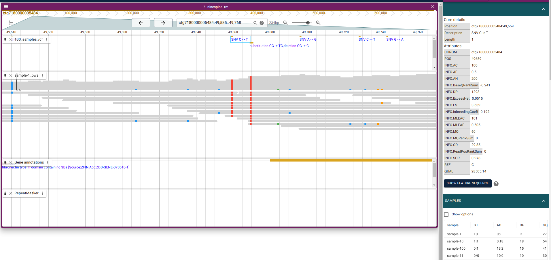
I’ve clicked the “SNV C->T” in the top of the panel (at position “ctg7180000005484:49659”) so that the panels on the right show the information for that variant: the upper panel shows the variant details and the lower panel the information for every sample. For “sample-1”, the information is the following:

sample	GT	AD	DP	GQ	PGT	PID	PL	PS
sample-1	1|1	0,9	9	27	1|1	49659_C_T	385,27,0	49659

The genotype (GT) is “1|1” meaning that “sample-1” is inferred to carry two “T” alleles. The allelic depth (AD) and the total depth (DP) of reads confirm that and report that zero “C” alleles and nine “T” alleles were found. This can be seen in the BAM panel:

BAM and VCF files.

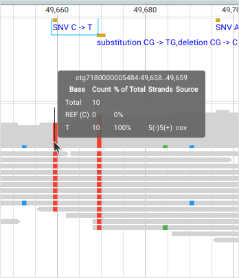
The vertical bars are reads (bottom) and each of them has a red square (“T” allele) at position “ctg7180000005484:49659”. The top part of the BAM panel shows the sequencing coverage and indicates that 10 reads carry the “T” allele. (The discrepancy of allelic depth, 9 vs. 10 copies, indicates that one of the reads have been later discarded.) The genotype quality (GQ) is given as a Phred score and “27” means that the chances of an erroneous genotype are close to 1/1000. As we’ll see later, the GQ value reappears in the Phred-scaled genotype likelihoods (PL). The variant ID (PID) comes from the position (PS) and the alleles.

While the JBrowse2 screenshot explains the connection between the reads (the BAM panel) and the variant calls (the VCF panel), it can only show the VCF information in the form of a separate table. The variant information across many samples is shown better in the IGV genome browser. IGV (https://igv.org/) comes as an old-school Java application that can be downloaded from here and run on personal computers, and as a web app.

If one opens the web app at https://popgeno.biocenter.helsinki.fi/igv-webapp/ and goes to the region “ctg7180000005484:49535-49768”, one can them click the top-most cyan block and open the information for “sample-1”

A VCF file in IGV.

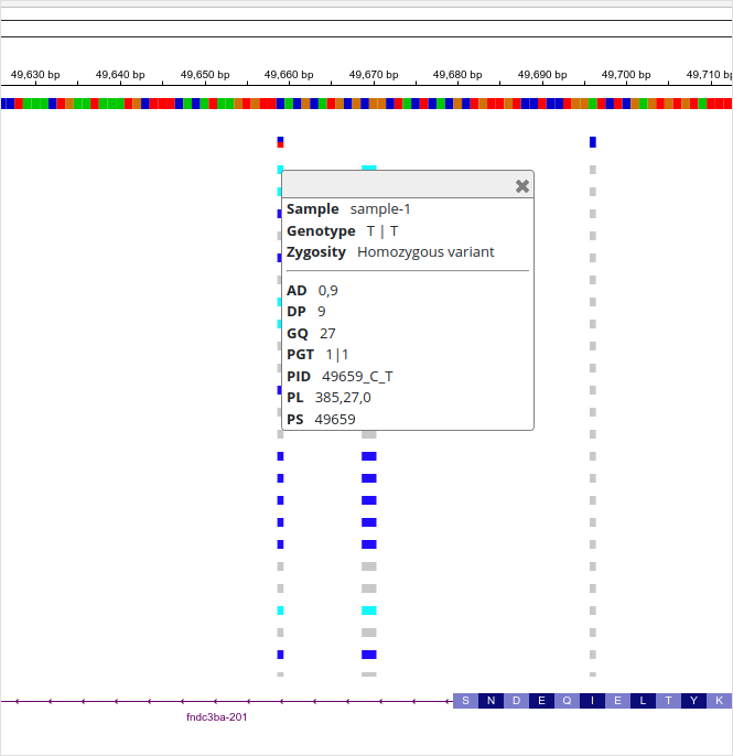
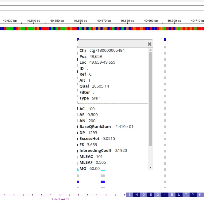
By clicking blocks of different colours, one learns that “cyan” means homozygous ALT, “blue” heterozygous and “grey” homozygous REF. The red-blue block on the top shows the summary of that position. Here, we see that the allele frequency (AF) is 0.50. This can be obtained by dividing the allele count (AC) by the total number of alleles (AN).

A VCF file in IGV.

Note that the panels can be adjusted by clicking the “Configuration” symbols on the extreme right of the window.

Own installation of IGV

Despite its age, the desktop version of IGV is still a highly useful program. Like JBrowse2, also IGV can read data from remote URLs, including the tunnelling approach explained in Own installation of JBrowse2.

Exercise: VCF variant position

The screenshot shows the information for one variant in contig “ctg7180000005484” for “sample-35”:

A VCF variant in IGV.

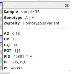
As the contig name is given, the figure contains all the information required to find the position in the IGV browser (or with bcftools view). Study the information at that position for “sample-1”.

Exercise 3 in Moodle.

A Swiss Army knife for VCF data

The program bcftools is by far the most important tool for anyone working on VCF data in a command-line environment. bcftools have so many subcommands that even an experienced user is unlikely to master all of them and knowing the just the central commands and options is a good start. However, those commands should be known by heart. Below is a collection of commands to start with. The program has a HOWTO page and a manual but unfortunately neither of those is aimed at beginners. On Puhti, bcftools is included e.g. in the “samtools” module.

Print out the subcommands and the help text for the subcommand “view”:

$ module load samtools

$ bcftools
$ bcftools view

Print out the VCF file header only, the contents without the header, and the full file:

$ vcf=vcfs/100_samples.vcf.gz

$ bcftools view -h $vcf | less -S
$ bcftools view -H $vcf | less -S
$ bcftools view $vcf | less -S

There are sometimes many ways to do the same. Print out the header again and study the difference:

 $ bcftools head $vcf | less -S
 $ bcftools view -h $vcf > 1
 $ bcftools head $vcf > 2
 $ diff 1 2

Many bcftools commands append the header with information about the processing steps. In ideal cases, the VCF header contains the full processing history of the data!

Print out region “ctg7180000005600:1000-2000” of “sample-10” without the header:

$ bcftools view -H -s sample-10 -r ctg7180000005600:1000-2000 $vcf | less -S

Print out the help text for bcftools query and pipe the previous bcftools view command to that using the example formatting from the help text. Note that the input VCF must contain the header and option -H cannot be used:

$ bcftools query
$ bcftools view -s sample-10 -r ctg7180000005600:1000-2000 $vcf | bcftools query -f '%CHROM\t%POS\t%REF\t%ALT[\t%SAMPLE=%GT]\n' -H | column -t

Do the same with bcftools query only:

$ bcftools query -s sample-10 -r ctg7180000005600:1000-2000 -f '%CHROM\t%POS\t%REF\t%ALT[\t%SAMPLE=%GT]\n' -H  $vcf | column -t

Print out region “ctg7180000005600:6000-7000” of “sample-10” with bcftools query formatting:

$ bcftools query -s sample-10 -r ctg7180000005600:6000-7000 -f '%CHROM\t%POS\t%REF\t%ALT[\t%SAMPLE=%GT]\n' -H  $vcf | column -t | less

For the same region, print out only variants of type “SNP” (-v snps) with exactly two alleles (-m2 -M2):

$ bcftools view -v snps -m2 -M2 -s sample-10 -r ctg7180000005600:6000-7000 $vcf | bcftools query -f '%CHROM\t%POS\t%REF\t%ALT[\t%SAMPLE=%GT]\n' -H | column -t | less

For the same region and sample, exclude sites with missing data (-g^miss). Note that this criterion has to be in a different command – after extracting “sample-10” – as some individuals have missing data on every site (the second command outputs nothing):

$ bcftools view -v snps -m2 -M2 -s sample-10 -r ctg7180000005600:6000-7000 $vcf | bcftools view -g ^miss | bcftools query -f '%CHROM\t%POS\t%REF\t%ALT[\t%SAMPLE=%GT]\n' -H | column -t | less
$ bcftools view -v snps -m2 -M2 -s sample-10 -r ctg7180000005600:6000-7000 -g^miss $vcf | bcftools query -f '%CHROM\t%POS\t%REF\t%ALT[\t%SAMPLE=%GT]\n' -H | column -t | less

For the same region, print out the alleles and their frequencies:

$ bcftools view -r ctg7180000005600:6000-7000 $vcf | bcftools query -f '%CHROM\t%POS\t%REF\t%ALT\t%INFO/AF\n' -H | column -t | less

For the same region, print out the alleles with different criteria on allele frequencies (AF) and minor allele frequencies (MAF):

$ bcftools view -i 'INFO/AF>0.05' -r ctg7180000005600:6000-7000 $vcf | bcftools query -f '%CHROM\t%POS\t%REF\t%ALT\t%INFO/AF\n' -H | column -t
$ bcftools view -i 'INFO/MAF>0.05' -r ctg7180000005600:6000-7000 $vcf | bcftools query -f '%CHROM\t%POS\t%REF\t%ALT\t%INFO/AF\n' -H | column -t
$ bcftools view -q 0.05 -Q 0.95 -r ctg7180000005600:6000-7000 $vcf | bcftools query -f '%CHROM\t%POS\t%REF\t%ALT\t%INFO/AF\n' -H | column -t
$ bcftools view -q 0.05:minor -r ctg7180000005600:6000-7000 $vcf | bcftools query -f '%CHROM\t%POS\t%REF\t%ALT\t%INFO/AF\n' -H | column -t
$ bcftools view -Q 0.95:major -r ctg7180000005600:6000-7000 $vcf | bcftools query -f '%CHROM\t%POS\t%REF\t%ALT\t%INFO/AF\n' -H | column -t

Note that the behaviour of these filtering options depends on the number of alternative alleles. If we only include binary variants (-m2 -M2), the output are identical:

$ bcftools view -m2 -M2 -i 'INFO/AF>0.05' -r ctg7180000005600:6000-7000 $vcf | bcftools query -f '%CHROM\t%POS\t%REF\t%ALT\t%INFO/AF\n' -H | column -t
$ bcftools view -m2 -M2 -i 'INFO/MAF>0.05' -r ctg7180000005600:6000-7000 $vcf | bcftools query -f '%CHROM\t%POS\t%REF\t%ALT\t%INFO/AF\n' -H | column -t
$ bcftools view -m2 -M2 -q 0.05 -Q 0.95 -r ctg7180000005600:6000-7000 $vcf | bcftools query -f '%CHROM\t%POS\t%REF\t%ALT\t%INFO/AF\n' -H | column -t
$ bcftools view -m2 -M2 -q 0.05:minor -r ctg7180000005600:6000-7000 $vcf | bcftools query -f '%CHROM\t%POS\t%REF\t%ALT\t%INFO/AF\n' -H | column -t
$ bcftools view -m2 -M2 -Q 0.95:major -r ctg7180000005600:6000-7000 $vcf | bcftools query -f '%CHROM\t%POS\t%REF\t%ALT\t%INFO/AF\n' -H | column -t

Important

When there are more than two alternative alleles, the behaviour of -q 0.05:minor may be unintuitive. For example, a position could have three variants with frequencies 0, 0.10 and 0.90. The position is clearly variable and not fixed to one allele. However, the minor allele frequency is 0 and -q 0.05:minor would discard it.

In the case of more than to alleles, nonmajor can be the more appropriate option. In the case here, these two commands give identical output:

$ bcftools view -q 0.05:nonmajor -r ctg7180000005600:6000-7000 $vcf | bcftools query -f '%CHROM\t%POS\t%REF\t%ALT\t%INFO/AF\n' -H | column -t
$ bcftools view -Q 0.95:major -r ctg7180000005600:6000-7000 $vcf | bcftools query -f '%CHROM\t%POS\t%REF\t%ALT\t%INFO/AF\n' -H | column -t

Print out regions “ctg7180000005600:1000-2000” and “ctg7180000005600:6800-6850” of “sample-10” and “sample-20” and format the output:

$ cat > samples.txt << EOF
sample-10
sample-20
EOF

$ echo -e "ctg7180000005600\t1000\t2000" >  regions.txt
$ echo -e "ctg7180000005600\t6800\t6850" >> regions.txt

$ bcftools query -S samples.txt -R regions.txt -f '%CHROM\t%POS\t%REF\t%ALT[\t%SAMPLE=%GT]\n' -H  $vcf | column -t

The formats for -S and -R are explained in the common options documentation.

Some useful picks from elsewhere. List the sample names:

$ bcftools query -l $vcf | head

Remove the QUAL, INFO and FORMAT fields; remove the header:

$ bcftools annotate --remove QUAL,INFO,FORMAT $vcf | bcftools view -H | less -S

There are some obvious (e.g. sort and index) and more specific (e.g. isec and csg) subcommands that we may use later. In the beginning, it is crucial to get familiar especially with view and the logic behind it. It doesn’t harm to split bcftools view command to many parts and sometimes it is strictly necessary.

The two commands below are equivalent; however, it is crucial that -r region comes first as it requires the index file that is available only for the input:

$ bcftools view -r ctg7180000005600:6000-7000 -v snps -m2 -M2 -s sample-10 $vcf \
  | bcftools query -f '%CHROM\t%POS\t%REF\t%ALT[\t%SAMPLE=%GT]\n' -H | column -t | less

$ bcftools view  -r ctg7180000005600:6000-7000 $vcf \
  | bcftools view -v snps \
  | bcftools view -m2 \
  | bcftools view -M2 \
  | bcftools view -s sample-10 \
  | bcftools query -f '%CHROM\t%POS\t%REF\t%ALT[\t%SAMPLE=%GT]\n' -H | column -t | less

Exercise: bcftools view command

Study the region 35000-45000 of the contig ctg7180000005484 in the file “vcfs/100_samples.vcf.gz” using the right options of bcftools view command.

Exercise 4 in Moodle.

Take-home message

In the variant calling of many samples, a common practice is to report the variants for a single sample in GVCF format that 1) lists the observed differences in comparison to the reference genome and 2) reports the certainty that there are truly no variants in the intervening positions. The latter is important as seeing no variants can be caused by the true lack of variants in the existing data and lack of data to observe the variants. GVCF information from many samples can be efficiently converted into VCF format: this retains only the variant positions and distinguishes sample sites being identical to the reference (“0/0”) from having no infromation (“./.”).

BAM and VCF files. BAM and VCF files. A VCF file in IGV. A VCF file in IGV. A VCF variant in IGV.