4. Working with BAM and VCF data

Learning outcome

After this practical, the students can describe and perform different approaches for VCF data filtering and subset VCF files to remove potential noise. They can perform PCA and distance-based clustering as exploratory analyses.

Getting to Puhti

Get to your working directory:

$ WORK=/scratch/project_2000598
$ cd $WORK/$USER

If you are on a login node (if you access Puhti through a stand-alone terminal, you get to a login node; in the web interface, you can select either a login node or a compute node), start an interactive job (see sinteractive -h for the options):

$ # the command below is optional, see the text!
$ sinteractive -A project_2000598 -p small -c 2 -m 4000 -t 8:00:00

Depending on the utilisation of the Puhti cluster, the last step may take time. If it doesn’t progress in a reasonable time (a couple of minutes), you may skip it and work on the login node. The work below is computationally light and should not put much strain on the login nodes.

Important

We will utilise the SLURM job scheduling system at Puhti. You can rehearse the vocabulary and concepts used at https://intscicom.biocenter.helsinki.fi/section5.html#running-jobs-on-a-linux-cluster

BAM quality control

samtools provides a command to compute basic statistics of BAM data and to plot these visually. We’ll do that for the first BAM file created by bwa mem and the final BAM file after the realignment:

$ cd $WORK/$USER
$ module load samtools
$ module load gnuplot

$ mkdir -p plots/bamstats

$ samtools stats bams/sample-1_bwa.bam > bams/sample-1_bwa.bamstats
$ plot-bamstats -p plots/bamstats/sample-1_bwa bams/sample-1_bwa.bamstats

$ samtools stats bams/sample-1_mdup.bam > bams/sample-1_mdup.bamstats
$ plot-bamstats -p plots/bamstats/sample-1_mdup bams/sample-1_mdup.bamstats

The output can be browsed as a text file:

$ less -S bams/sample-1_bwa.bamstats

However, it is more useful in the form of plots. You can see those plots in a web browser by starting a Jupyter session at https://www.puhti.csc.fi/ and then finding the output directory “/scratch/project_2000598/username/plots/bamstats/”. An alternative is to got to https://www.puhti.csc.fi/ and select “Files” from the top bar. However, that can only show the graphics files, not the HTML file.

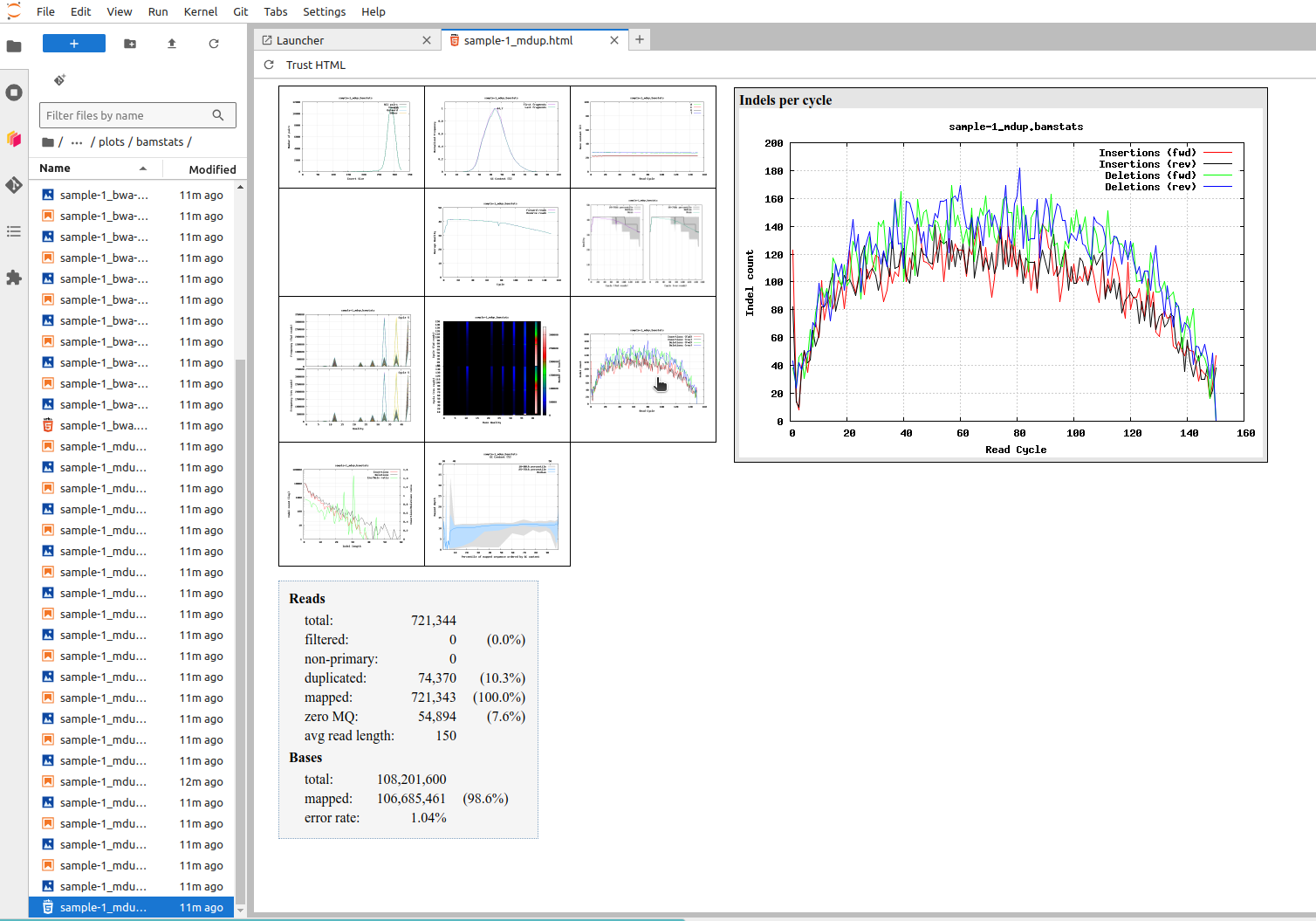
In the Jupyter file browser, locate and open the file “sample-1_mdup.html”. You can then point the small plots on the left to open them in the right.

The first plot shows the insert size, the length of the fragments that are sequenced from both ends. The mean length is just below 300 bp meaning that the 150 bp-long reads from the two ends slightly overlap in the middle. The next two plots are the CG content and the base content, and it is easy to see that the numbers are consistent.

The second row plots visualise the base quality across the read positions. We see two things: the first few bases tend to be poor and the quality slowly deteriorates after position 100. Sometimes the backwards read is of poorer quality than the forward read as it is generated last.

The next interesting plot is about “Indels per cycle”, shown in the picture. It is useful to compare that plot to one about “Per-base sequence content”. The latter shows the frequency of A, C, G and T at different positions of the reads (flat as they should be) while the former frequency of insertions and deletions at different positions. One would think that, like the bases, indels would be equally likely at every position but that doesn’t seem to be the case.

There are two reasons for that: a comparison of the plots for “sample-1_bwa” and “sample-1_mdup” reveals that the use GATK IndelRealigner has created new indels at the very first positions, suggesting that bwa mem has made errors in the mapping and has not made indels in the very ends of the reads. The reason for that is in the scoring function:

Scoring options:

       -A INT        score for a sequence match, which scales options -TdBOELU unless overridden [1]
       -B INT        penalty for a mismatch [4]
       -O INT[,INT]  gap open penalties for deletions and insertions [6,6]
       -E INT[,INT]  gap extension penalty; a gap of size k cost '{-O} + {-E}*k' [1,1]
       -L INT[,INT]  penalty for 5'- and 3'-end clipping [5,5]
       -U INT        penalty for an unpaired read pair [17]

The penalty for a mismatch is -4 while that for an indel is -6. The score for a match is +1, meaning that several matches are needed to compensate for an indel if the alternative is creating a mismatch.

The more important reason is that the penalty for end clipping is only -5. If an indel is towards the end of the read, a better total mapping score can often be obtained by not opening an indel and then making a few matches but simply by clipping the end of the read and throwing it away.

The details of this are not super important but it is good to remember that short-read sequencing is much better in identifying independent SNPs than complex indels.

Exercise: Read clipping

The BAM file bams/sample-1_mdup.bam contains clipped reads in the contig “ctg7180000005484” between positions 95430 and 95440. You can visualise them using samtools tview or JBrowse2.

Several reads have been clipped on their left end at exactly the same position. What is the first genome position where the clipped reads have retained the sequence?

Exercise 1 in Moodle.

VCF filtering

Our full data contain 279,512 variants:

$ bcftools index vcfs/100_samples.vcf.gz
$ bcftools index -n vcfs/100_samples.vcf.gz

It is impossible to provide “correct” criteria for filtering VCF data and we here go through some possibilities. We first remove variants that are in the proximity of indels (-g 20) and then select binary SNPs (-m2 -M2 -v snps) and finally remove variants within repeat elements (-T ^reference/ninespine_rm.gff.gz) and keep those within the positively masked regions (-T reference/ninespine_posmask.bed.gz):

$ bcftools filter -g 20 vcfs/100_samples.vcf.gz | \
    bcftools view -m2 -M2 -v snps -T ^reference/ninespine_rm.gff.gz \
    -T reference/ninespine_posmask.bed.gz -Oz -o vcfs/100_samples_rpm_snps.vcf.gz
$ bcftools index vcfs/100_samples_rpm_snps.vcf.gz
$ bcftools index -n vcfs/100_samples_rpm_snps.vcf.gz

These steps reduce the number of variants to 128,987. If you struggle to understand the commands, see the help texts for bcftools filter and bcftools view and return to introduction to bcftools in the previous section.

Defining regions in VCF files

The command bcftools view gives the description of the command options and these include -r, -R, -t and -T:

    -r, --regions REGION              Restrict to comma-separated list of regions
    -R, --regions-file FILE           Restrict to regions listed in FILE
    -t, --targets [^]REGION           Similar to -r but streams rather than index-jumps. Exclude regions with "^" prefix
    -T, --targets-file [^]FILE        Similar to -R but streams rather than index-jumps. Exclude regions with "^" prefix

With the lower-case letters one gives the region in the command and with the capital letters one specifies a file that list the regions. But what is the practical difference between -R and -T?

Let’s imagine that one would need to fetch books from a library. The books are ordered alphabetically by the name and the right shelf can be found from an “index”, a list describing the shelves for books with names starting with a specific letter.

The option -R is similar to having the list of books to fetch on a table and then checking the place of one book at a time from the index and walking to fetch the book from the shelf. That works fine for a small number of books that we typically borrow from a library.

What if we would need to fetch thousands of books? That would make a lot walking back and forth!

The option -T is similar to having the list of books to fetch in hand and walking through the entire library from the first shelf to the last one and checking every book against the list of books to take. If the book is on the list, it is taken, otherwise not.

It is easy to see that one option is better for a handful of books and the other for a huge number of books, but it is not easy to say at which number of books one approach becomes better than the other. In the commands above, it is clear that -T is far superior to define a large number of regions across the whole genome.

The beauty of the two options is that they can be combined. If we would need to fetch thousands of books with names starting with letters K and L, it would be wasteful to walk through the entire library from A to Ö. In that case, we we could use -R (or -r) to define the shelves containing K and L and then -T to define the books to collect.

These criteria seem strict but the next steps reveal that the data contain problematic sites. We first output the total mapping coverage (across all samples) of each variant:

$ bcftools query -f '%CHROM,%POS,%DP\n' vcfs/100_samples_rpm_snps.vcf.gz > vcfs/100_samples_rpm_snps.csv

We then analyse these in R (you can use RStudio at https://www.puhti.csc.fi):

setwd(paste0("/scratch/project_2000598/",Sys.getenv("USER")))

dat <- read.csv("vcfs/100_samples_rpm_snps.csv")
colnames(dat) <- c("ctg","pos","depth")
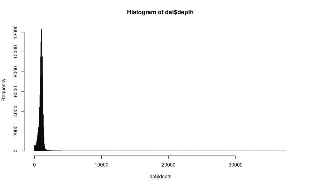
hist(dat$depth,breaks=1000)
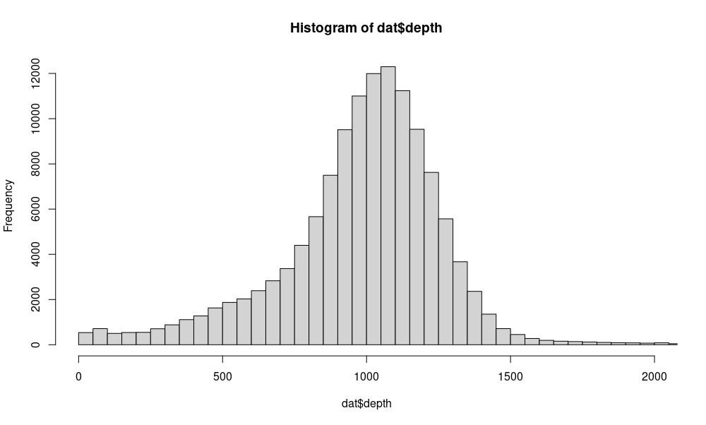
hist(dat$depth,breaks=1000,xlim=c(0,2000))

R and RStudio on Puhti

Puhti provides both the command-line version of R and the graphical RStudio. R can only be run on a compute node (either selecting “Compute node shell” or starting one with sinteractive). It is then started with:

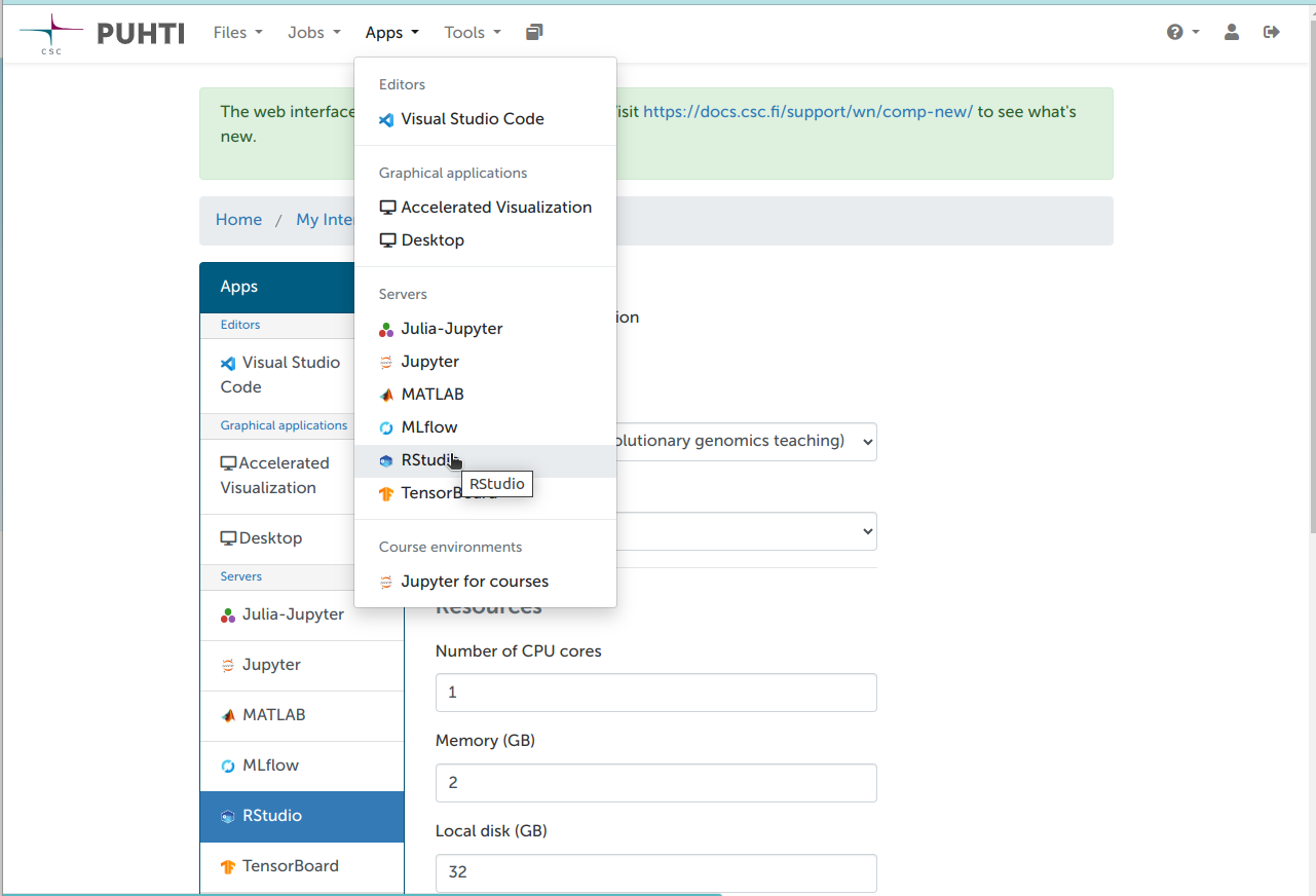
$ module load r-env
$ start-r

RStudio is started from https://www.puhti.csc.fi):

The students are expected to know the basics of R and RStudio.

We can see that the maximum sequencing depth is 37,577 but typically the total depth varies around 1,000. (Can you see why that is the case?)

Based on that, we keep (-i 'INFO/DP>400 && INFO/DP<1800') only sites with total depth between 400 and 1800:

$ bcftools view -i 'INFO/DP>400 && INFO/DP<1800' -Oz -o vcfs/100_samples_rpm_snps_dpt.vcf.gz vcfs/100_samples_rpm_snps.vcf.gz
$ bcftools index vcfs/100_samples_rpm_snps_dpt.vcf.gz
$ bcftools index -n vcfs/100_samples_rpm_snps_dpt.vcf.gz

This retains 121,169 variants.

The number of singletons, i.e. variants found heterozygous in one sample only, is informative of the population size and history. However, the number of singletons is also potentially misleading when analysing low-coverage data where the power to detect alleles present only once is low. In many analyses, rare alleles are not utilised or their impact is miniscule, and it is a common practice to remove variants whose frequency is below a threshold. A second common practice is to remove sites at which many samples lack data – or have “missing data”.

With bcftools view, one can set a lower and upper limit for the allele frequency with options -q and -Q. If we would set the minimum allele frequency (MAF) of 5%, we could then say -q 0.05 -Q 0.95. However, it is simpler to specify the same as -q 0.05:minor. The amount of missing data is a feature that we can usitise in a condition and then either include -i or exclude -e sites that do not fulfill that condition. We can include sites with less than 10% missing data with the option -i 'F_MISSING<0.1'. This gives us the command:

$ bcftools view -i 'F_MISSING<0.1' -q 0.05:minor -Oz -o vcfs/100_samples_rpm_snps_dpt_maf.vcf.gz vcfs/100_samples_rpm_snps_dpt.vcf.gz
$ bcftools index vcfs/100_samples_rpm_snps_dpt_maf.vcf.gz
$ bcftools index -n vcfs/100_samples_rpm_snps_dpt_maf.vcf.gz

and retains 48,686 variants.

Important

When there are more than two alternative alleles, the behaviour of -q 0.05:minor may be unintuitive. For example, a position could have three variants with frequencies 0, 0.10 and 0.90. The position is clearly variable and not fixed to one allele. However, the minor allele frequency is 0 and -q 0.05:minor would discard it.

The documentation for -q is the following:

    -q/Q, --min-af/--max-af FLOAT[:TYPE]   Minimum/maximum frequency for non-reference (nref), 1st alternate (alt1), least frequent
                                               (minor), most frequent (major) or sum of all but most frequent (nonmajor) alleles [nref]

Based on that, -q 0.05:nonmajor may sometimes be the more appropriate option.

Another common property to check in the quality control is the Hardy-Weinberg equilibrium. A typical error in variant data is that the reads belonging to different but highly similar genome regions (e.g. different repeat elements or different copies of segmental duplicate regions) are mapped to one copy only. If that happens, the few differences between the copies (e.g. repeat elements) create fake heterozygous positions; as all/most individuals carry the conflicting copies, heterozygotes are massively overrepresented. An excess of heterozygous can be detedcted with a statistical test and sites with extreme p-values can be discarded. The HWE test is not bcftools but is included in vcftools. The latter can read and write VCF files but does it more slowly than bcftools and a common practice is to pipe the data between the commands (you may find out how to do it with vcftools only):

$ module load vcftools
$ bcftools view vcfs/100_samples_rpm_snps_dpt_maf.vcf.gz | \
    vcftools --vcf - --hwe 0.000001 --recode --recode-INFO-all --stdout | \
    bcftools view -Oz -o vcfs/100_samples_rpm_snps_dpt_maf_hwe.vcf.gz
$ bcftools index vcfs/100_samples_rpm_snps_dpt_maf_hwe.vcf.gz
$ bcftools index -n vcfs/100_samples_rpm_snps_dpt_maf_hwe.vcf.gz

That reduces the number of variants to 33,875.

( Unlike bcftools, the program vcftools doesn’t provide a summay of the program options. The documentation and manual for vcftools can be found at its GitHub page. )

Finally, the variant set can be thinned such that variants close to each other are removed. Thinnig by distance can be done e.g. with vcftools and plink, the latter also providing options to randomly select a specific number of sites. We do the thinning with plink and set the minimum distance at 1000 bp:

$ module load plink/1.90
$ plink --vcf vcfs/100_samples_rpm_snps_dpt_maf_hwe.vcf.gz --allow-extra-chr --bp-space 1000 --recode vcf bgz --out vcfs/100_samples_rpm_snps_dpt_maf_hwe_thin
$ bcftools index vcfs/100_samples_rpm_snps_dpt_maf_hwe_thin.vcf.gz
$ bcftools index -n vcfs/100_samples_rpm_snps_dpt_maf_hwe_thin.vcf.gz

All the filtering put together retains only 5,824 variants.

( The documentation for plink v.1.9 is available at https://www.cog-genomics.org/plink. The version 1.9 and 2.0 differ and all program options and functions are not found in both versions. )

Exercise: Read filtering

Three files are available at: bash $ ls $WORK/shared/moodle/ctg_filter[ABC].vcf.gz

One of these was generated by filtering the original data using a minimum allele frequency threshold (“XX” below) of either 0.05, 0.10 or 0.20; another file was generated with the threshold for missing data (“YY”) set either at 0.05, 0.10 or 0.20; a third file was generated by combining the two previous criteria.

The commands used were:

$ bcftools view -qXX:minor full.vcf.gz
$ bcftools view -i 'F_MISSING<YY' full.vcf.gz
$ bcftools view -qXX:minor -i 'F_MISSING<YY' full.vcf.gz

Which command was used for which file?

Exercise 2 in Moodle.

Visual view on variant filtering

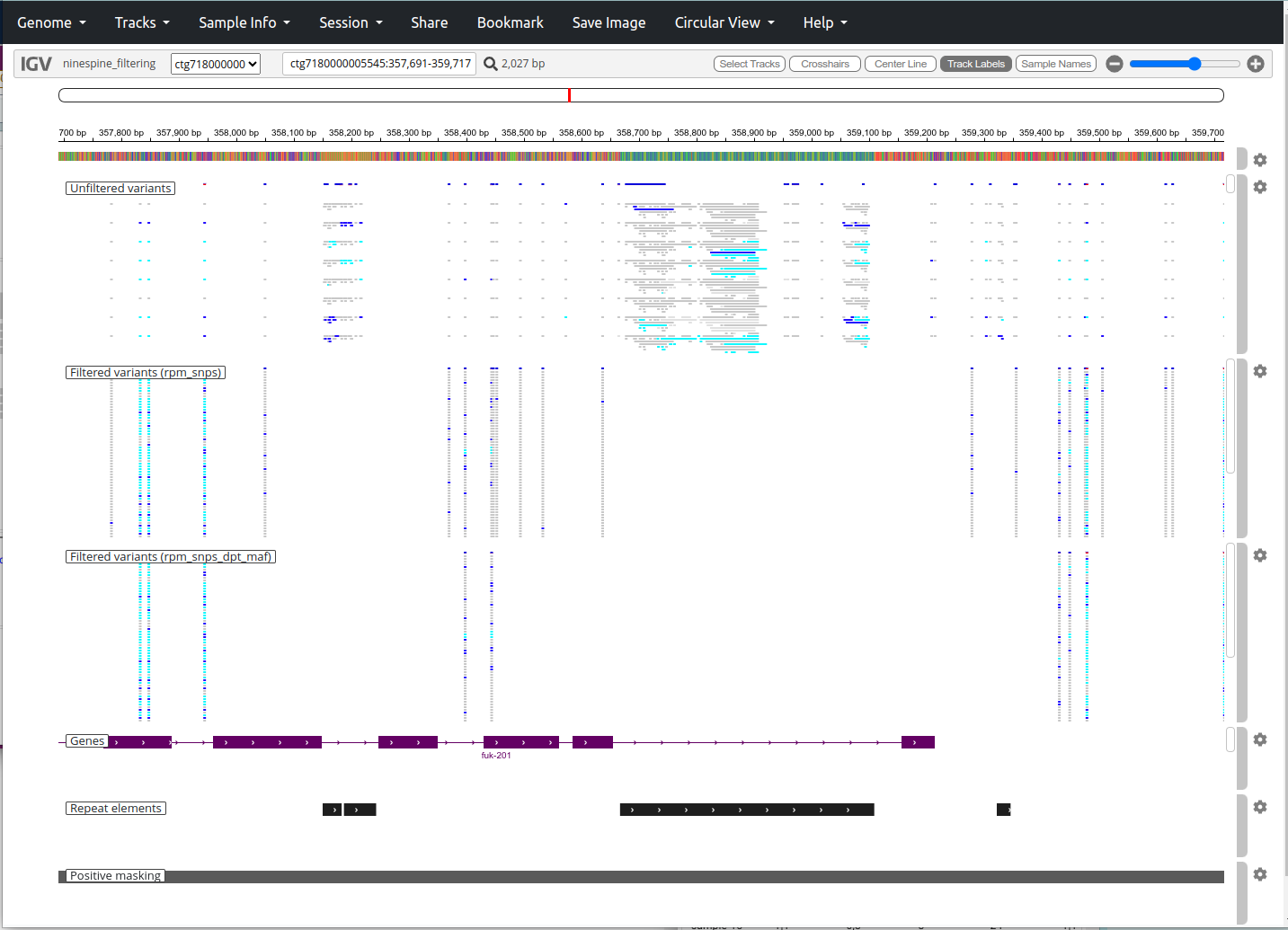
The impact of VCF filtering can be seen in a genome browser. The IGV browser at https://popgeno.biocenter.helsinki.fi/igv-webapp/ has an alternative genome “ninespine draft-genome, partial (2)” in the “Genome” pull-down menu in the top-left corner. If you then go to the location “ctg7180000005545:357691-359717”, the view should be like this:

In the top-panel, we have the full variant data, “100_samples.vcf.gz”; in the mid-panel, we have the minimally filtered SNP set, “100_samples_rpm_snps.vcf.gz”; and in the bottom-panel, we have the slightly more filtered, “100_samples_rpm_snps_dpt_maf.vcf.gz”.

The greatest difference is between the two top-most panels where the removal of indels removes the overlapping variants and makes the two lower panels more table-like. We can also see that the two large repeat element regions (marked at the bottom) have lots of “variants” in the top panel and all these have been discarded by removing the repeat masked regions and including only the positively masked regions. The difference between the two lower panels is mostly by the MAF filtering: we can see that the variants missing from the bottom panel contain rare alleles in the mid-panel (most genotypes are grey, meaning REF; a few are blue, meaning hetrozygote).

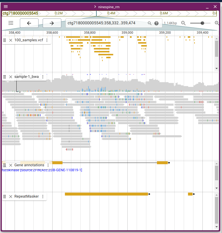
The reason for discarding the repeat element regions can be seen in the JBrowse2:

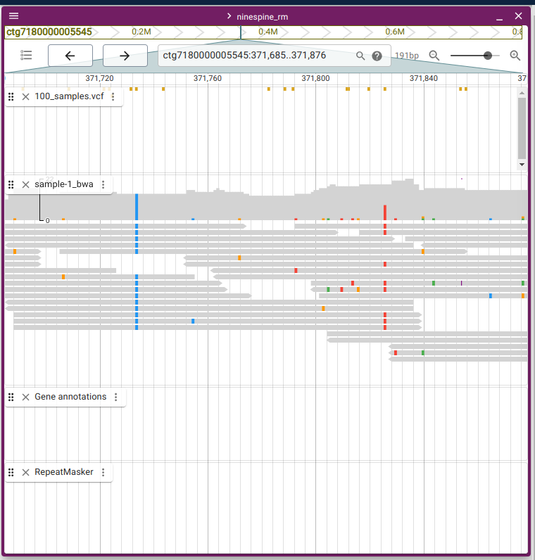
The two regions are at “ctg7180000005545:358332-359474” and “ctg7180000005545:371685-371876”.

In the left picture, the reads (sample-1_bwa.bam) mapped to the repeat region (RepeatMasker) contain huge numbers of differences (coloured blocks in grey reads) and produce numerous “variants” (100_samples.vcf.gz). The inconsistency of the reads reveals that they cannot be from the same source.

The right picture shows a trustworthy region: the variant is present in all reads (left, in blue) if it is homozygous, or in roughly half of the reads (right, in red) if it is heterozygous. The reads contain base calling errors but they do not produce a consistent pattern.

A visual browser is often useful but it is normally more efficient to view data using command-line tools. The good region can be viewed with samtools tview with the command:

$ samtools tview bams/sample-1_mdup.bam reference/ninespine_rm.fa -p ctg7180000005545:371695

The genotypes can be viewed with bcftools view but the full output can be messy. This shows the same region as the samtools tview command above and we can see that the genotypes are “1/1” and “0/1” (they are at the ends of the lines):

$ bcftools view -H -q 0.1 -s sample-1 -r ctg7180000005545:371730-371830 vcfs/100_samples_rpm_snps.vcf.gz

ctg7180000005545    371733  .   T   C   9593.54 PASS    AC=2;AF=0.444;AN=2;BaseQRankSum=0;DP=473;ExcessHet=0;FS=4.978;InbreedingCoeff=0.6122;MLEAC=90;MLEAF=0.634;MQ=48.54;MQRankSum=-0.712;QD=31.75;ReadPosRankSum=-1.383;SOR=0.358    GT:AD:DP:GQ:PGT:PID:PL:PS   1/1:0,10:10:30:.:.:383,30,0:.
ctg7180000005545    371825  .   C   T   7299.88 PASS    AC=1;AF=0.551;AN=2;BaseQRankSum=0.524;DP=551;ExcessHet=0;FS=5.594;InbreedingCoeff=0.4203;MLEAC=108;MLEAF=0.794;MQ=49.06;MQRankSum=-2.638;QD=30.16;ReadPosRankSum=-0.303;SOR=1.09    GT:AD:DP:GQ:PL  0/1:9,4:13:99:134,0,296

bcftools query allows showing only the fields of interest:

$ bcftools query -i 'INFO/MAF>0.1' -r ctg7180000005545:371730-371830 -s sample-1 -f '%CHROM\t%POS\t%REF\t%ALT[\t%GT]\n' vcfs/100_samples_rpm_snps.vcf.gz

ctg7180000005545    371733  T   C   1/1
ctg7180000005545    371825  C   T   0/1

In the examples above, the MAF filters are used to discard the SNP sites not variable in “sample-1”. Type bcftools query to see the help text of the command.

Using the same approach, we can compare the set of variants retained in a table format:

$ bcftools query -r ctg7180000005545:358300-358700 -f '%CHROM\t%POS\t%REF\t%ALT[\t%GT]\n' vcfs/100_samples_rpm_snps.vcf.gz | less -S
$ bcftools query -r ctg7180000005545:358300-358700 -f '%CHROM\t%POS\t%REF\t%ALT[\t%GT]\n' vcfs/100_samples_rpm_snps_dpt_maf.vcf.gz | less -S

One can see that the sites include only in the first file are mostly of genotype “0/0”.

That can be confirmed by plotting the allele frequencies (“INFO/AF”):

$ bcftools query -r ctg7180000005545:358300-358700  -f '%CHROM\t%POS\t%REF\t%ALT\t%INFO/AF\n' vcfs/100_samples_rpm_snps.vcf.gz

ctg7180000005545    358370  G   T   0.035
ctg7180000005545    358398  G   T   0.085
ctg7180000005545    358444  C   G   0.135
ctg7180000005545    358447  C   T   0.005
ctg7180000005545    358453  G   A   0.005
ctg7180000005545    358494  C   G   0.005051
ctg7180000005545    358533  C   T   0.005
ctg7180000005545    358637  G   A   0.01

Two VCF files can also be compared with bcftools isec. The resulting README file explains the VCF-formatted output:

$ mkdir vcfs/isec
$ bcftools isec -p vcfs/isec -Oz vcfs/100_samples_rpm_snps.vcf.gz vcfs/100_samples_rpm_snps_dpt_maf.vcf.gz
$ less -S vcfs/isec/README.txt

This file was produced by vcfisec.
The command line was:   bcftools isec  -p vcfs/isec -Oz vcfs/100_samples_rpm_snps.vcf.gz vcfs/100_samples_rpm_snps_dpt_maf.vcf.gz

Using the following file names:
vcfs/isec/0000.vcf.gz  for records private to  vcfs/100_samples_rpm_snps.vcf.gz
vcfs/isec/0001.vcf.gz  for records private to  vcfs/100_samples_rpm_snps_dpt_maf.vcf.gz
vcfs/isec/0002.vcf.gz  for records from vcfs/100_samples_rpm_snps.vcf.gz shared by both        vcfs/100_samples_rpm_snps.vcf.gz vcfs/100_samples_rpm_snps_dpt_maf.vcf.gz
vcfs/isec/0003.vcf.gz  for records from vcfs/100_samples_rpm_snps_dpt_maf.vcf.gz shared by both        vcfs/100_samples_rpm_snps.vcf.gz vcfs/100_samples_rpm_snps_dpt_maf.vcf.gz

In addition to that, it produces file “vcfs/isec/sites.txt” that we can index and then study the region of interest:

$ bgzip vcfs/isec/sites.txt 
$ tabix -s1 -b2 -e2 vcfs/isec/sites.txt.gz 
$ tabix vcfs/isec/sites.txt.gz ctg7180000005545:358300-358700

ctg7180000005545    358370  G   T   10
ctg7180000005545    358398  G   T   11
ctg7180000005545    358444  C   G   11
ctg7180000005545    358447  C   T   10
ctg7180000005545    358453  G   A   10
ctg7180000005545    358494  C   G   10
ctg7180000005545    358533  C   T   10
ctg7180000005545    358637  G   A   10

The last column indicates whether the site was included in (1) or missing from (0) the first and second file, respectively. In this region only two sites are shared between the files (“11”).

Exercise: Difference between two VCF files

The file $WORK/shared/moodle/ctg_dpt_maf_sites.txt start like this:

ctg7180000005484    18874   C   T   10
ctg7180000005484    18890   A   G   11
ctg7180000005484    18917   C   A   11
ctg7180000005484    18969   G   T   11
ctg7180000005484    19030   T   A   11
ctg7180000005484    19163   A   G   11

and contains the summary of the command:

$ bcftools isec $WORK/shared/moodle/ctg_rpm_snps_dpt.vcf.gz $WORK/shared/moodle/ctg_rpm_snps_maf.vcf.gz -p isec

Find out how many variants are unique to the two files and how many are shared. This can be done using the ctg_dpt_maf_sites.txt file only or rerunning the bcftools isec command.

Exercise 3 in Moodle.

Exploratory statistics

The aim of exploratory analyses is to confirm that the data production and processing have been successful and no obvious mistakes have been done. They also get a first glimpse on the general properties of the data and can guide the subsequent “proper” analyses.

We look at two simple methods, Principal Component Analysis (PCA) and Clustering.

PCA

We use plink for the PCA and to compute pairwise distances for clustering. PCA is done by specifying the option --pca. Instead of distances, plink only provides identities (IBS = Identity By State) and we have to select option 1-ibs to conver them to distances; we additionally select square and gz to get the values as a square matrix (not trinagular) and to compress the output. The last one is not significant here but can be useful with larger datasets.

The population identities of different samples is provided in the file “sample_names.txt”. For illustrative purposes, we do the PCA for a minimally filtered set of data and for a heavily filtered set of data:

$ mkdir plink
$ cp $WORK/shared/data/sample_names.txt plink/

$ plink --vcf vcfs/100_samples_rpm_snps.vcf.gz --allow-extra-chr --pca \
    --distance 1-ibs square gz --out plink/100_samples_rpm_snps
$ plink --vcf vcfs/100_samples_rpm_snps_dpt_maf_hwe_thin.vcf.gz --allow-extra-chr --pca \
    --distance 1-ibs square gz --out plink/100_samples_rpm_snps_dpt_maf_hwe_thin

We can see the output matrix:

$ cat plink/100_samples_rpm_snps.eigenvec | column -t | less -S

The file *.eigenvec and *.eigenval are the eigenvectors and eigenvalues. The eigenvectors are the axes of the principal component transformation and the eigenvalues tell the amount of variance that these axes explain (see Wikipedia). The components are ordered such that the component explaining most of the variation comes first and the others in the order of decreasing importance.

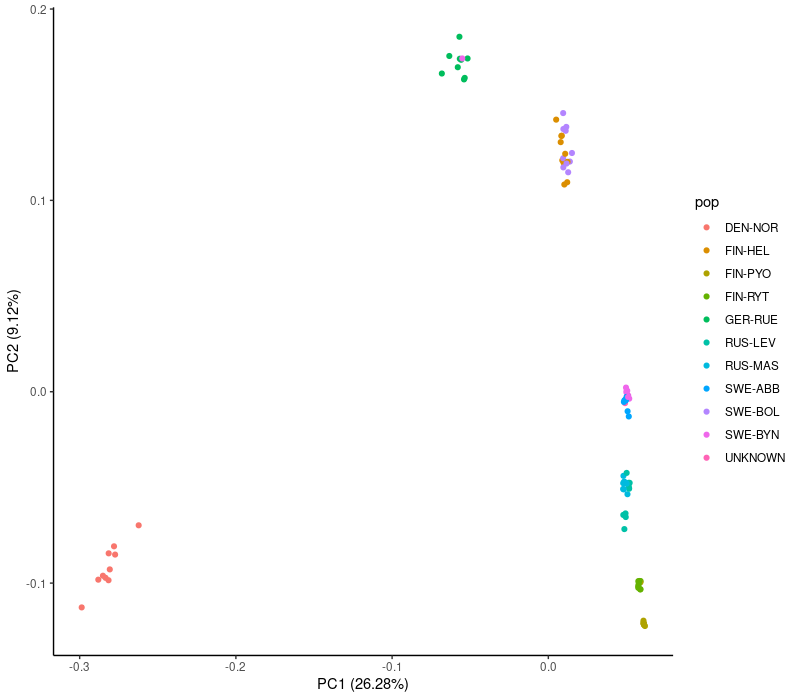
We process the PCA data in R/Rstudio. Here we plot the first two principal components and add the proportion of the variance that these axes explain in the axis labels:

setwd(paste0("/scratch/project_2000598/",Sys.getenv("USER")))

library(ggplot2) 

pops <- read.table("plink/sample_names.txt", col.names = c("pop","smp"))

vec <- read.table("plink/100_samples_rpm_snps.eigenvec",col.names = c("smp","pop",paste0("PC",1:20)))
vec$pop <- pops$pop[match(vec$smp,pops$smp)]

val <- read.table("plink/100_samples_rpm_snps.eigenval",header=F)[,1]
lab1 <- paste0("PC1 (",round(val[1]/sum(val)*100,2),"%)")
lab2 <- paste0("PC2 (",round(val[2]/sum(val)*100,2),"%)")

ggplot() + 
    geom_point(data=vec,aes(PC1,PC2,color=pop)) + 
    geom_point(data=subset(vec,smp=="sample-1"),aes(PC1,PC2),color="black") + 
    xlab(lab1) + ylab(lab2) +
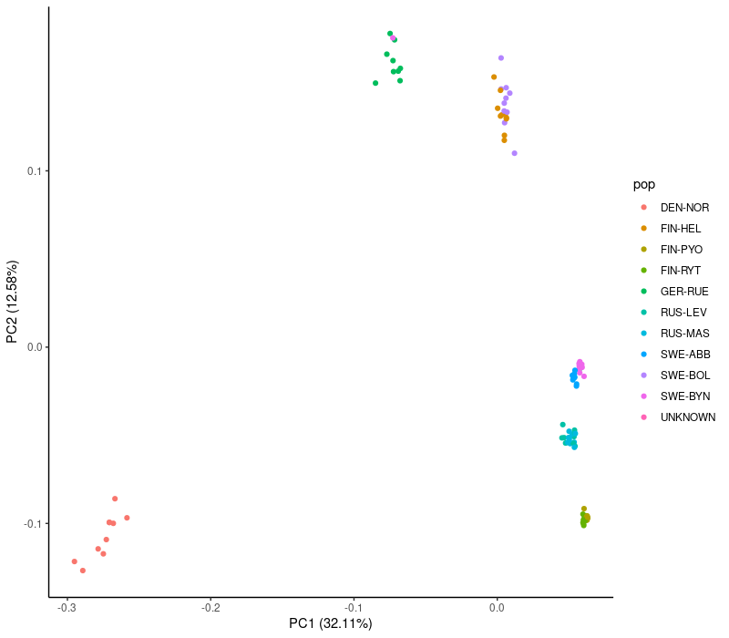
    theme_classic()

This was for the larger (127,987 SNPs) data set. Note that “sample-1” is replotted in black to make it visible.

The same for the smaller (5,824 SNPs) data set is done as:

vec <- read.table("plink/100_samples_rpm_snps_dpt_maf_hwe_thin.eigenvec",col.names = c("smp","pop",paste0("PC",1:20)))
vec$pop <- pops$pop[match(vec$smp,pops$smp)]

val <- read.table("plink/100_samples_rpm_snps_dpt_maf_hwe_thin.eigenval",header=F)[,1]
lab1 <- paste0("PC1 (",round(val[1]/sum(val)*100,2),"%)")
lab2 <- paste0("PC2 (",round(val[2]/sum(val)*100,2),"%)")

ggplot() + 
    geom_point(data=vec,aes(PC1,PC2,color=pop)) + 
    geom_point(data=subset(vec,smp=="sample-1"),aes(PC1,PC2),color="black") + 
    xlab(lab1) + ylab(lab2) +
    theme_classic()

We see that the PCA plots are largely similar and group many of the populations. Those with sharp eyes may notice a change in the bottom right corner: the heavily filtered data fails to separate the two populations there, possibly because the MAF filter removed rare variants specific to these populations. There are a few other oddities but we look at those later.

Clustering

plink converted sequence identities (1-ibs) to produce pairwise genetic distances, and we use a clustering algorithm to produce tree from these distances. Before that, we have a look on what we have:

$ less -S plink/100_samples_rpm_snps.mdist.id
$ zcat plink/100_samples_rpm_snps.mdist.gz | column -t | less -S

We use the neighbour joining (NJ) algorithm to cluster our data. The algorithm is nicely explained in the Wikipedia.

Generally, a tree is not a very good approach for visualising population genetic data as the data as a whole has not evolved in a tree-like manner. Every single site in the genome has a history that can be represented as a tree, but the genomes undergo recombination and different parts of the genome thus have evolved under different trees. The distance data represent this cacophony of conflicting signals, but it is not guaranteed to produce a meaningful “average” of the different histories.

Despite the potential problems, clustering trees are useful tools for exploratory analyses and some parts of the result can be trusted. The NJ algorithm is included in the R package “ape” which is included in the package “ggtree”. We use midpoint rooting to place the Atalntic population (DEN-NOR) as the outgroup to the Fennoscandian populations:

setwd(paste0("/scratch/project_2000598/",Sys.getenv("USER")))

library(ggtree) 
library(phangorn)

pops <- read.table("plink/sample_names.txt", col.names = c("pop","smp"))
pops$smp <- gsub("-",".",pops$smp)

nms <- read.table("plink/100_samples_rpm_snps.mdist.id", header=F,sep="\t")[,1]
dst <- read.table("plink/100_samples_rpm_snps.mdist.gz", header=F,sep="\t",col.names=nms, fill=T)

njt <- nj(as.dist(dst))
njt.rt <- midpoint(njt)

tip.col <- factor(pops$pop[match(njt.rt$tip.label,pops$smp)],labels=rainbow(11))

njt.rt$tip.label <- paste(njt.rt$tip.label,pops$pop[match(njt.rt$tip.label,pops$smp)])

ggtree(njt.rt, ladderize=TRUE, size=0.25) +
 geom_tiplab(align=T, linetype = "dotted", linesize=0.25, size=1, color=tip.col) +
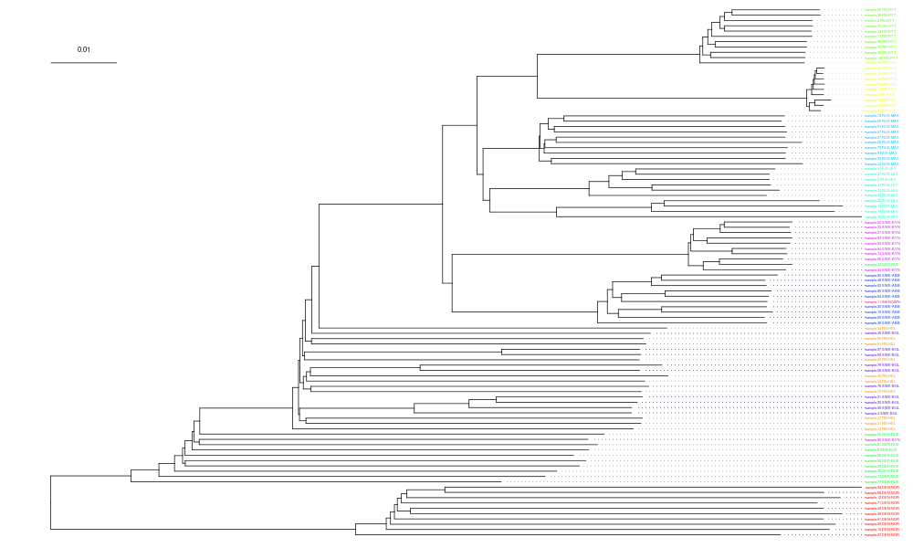
 geom_treescale(x=0,y=90,fontsize=2,linesize=0.25,offset=2)

The tree labels are impossible read in this figure but the colours show that many of the populations are clustered together.

Important

The plots generated within RStudio can be saved as graphics files using the options in the “Plots” tab in the bottom right menu bar. The file system can be browsed – and graphics files viewed – through the “Files” tab. The pdf format allows zooming into small details.

Plots and trees with R’s base graphics

The R package “ggtree” works in the style of “ggplot2” and those familiar with the latter may find it intuitive. Those more familiar with the base graphics can stick to that and do the plots in the old style.

The PCA plot can be produced e.g. like this:

setwd(paste0("/scratch/project_2000598/",Sys.getenv("USER")))

pops <- read.table("plink/sample_names.txt", col.names = c("pop","smp"))

vec <- read.table("plink/100_samples_rpm_snps.eigenvec",col.names = c("smp","pop",paste0("PC",1:20)))
vec$pop <- pops$pop[match(vec$smp,pops$smp)]
col <- as.character(factor(vec$pop,labels=rainbow(11)))

val <- read.table("plink/100_samples_rpm_snps.eigenval",header=F)[,1]
lab1 <- paste0("PC1 (",round(val[1]/sum(val)*100,2),"%)")
lab2 <- paste0("PC2 (",round(val[2]/sum(val)*100,2),"%)")

plot(vec$PC1,vec$PC2,col=col,xlab=lab1,ylab=lab2,pch=20)

and the clustering tree like this:

setwd(paste0("/scratch/project_2000598/",Sys.getenv("USER")))

library(ape) 
library(phangorn)

pops <- read.table("plink/sample_names.txt", col.names = c("pop","smp"))
pops$smp <- gsub("-",".",pops$smp)

nms <- read.table("plink/100_samples_rpm_snps.mdist.id", header=F,sep="\t")[,1]
dst <- read.table("plink/100_samples_rpm_snps.mdist.gz", header=F,sep="\t",col.names=nms, fill=T)

njt <- nj(as.dist(dst))
njt.rt <- midpoint(njt)

tip.col <- factor(pops$pop[match(njt.rt$tip.label,pops$smp)],labels=rainbow(11))

njt.rt$tip.label <- paste(njt.rt$tip.label,pops$pop[match(njt.rt$tip.label,pops$smp)])

plot(njt.rt,cex=0.25,tip.color = as.character(tip.col))
add.scale.bar()

Exercise: Exploratory analyses

The PCA and clustering plots provide the first glimpses on the data. If the sequencing or processing of an individual sample has failed, the sample shows up as an outlier in the PCA and the clustering tree.

In our study, we have processed “sample-1” and combined it with 99 other samples. The metadata for other samples are available but the origin of “sample-1” is not given. With the exploratory analyses performed, identifying the population of origin is trivial.

The data are a subset of the original data. In the original data, some samples were mislabelled and they now group with wrong samples. With the exploratory analyses performed, they can also be identified.

Exercise 4 in Moodle.

Take-home message

Unfortunately, there are no perfect guidelines and instructions for variant filtering. Many population genetics inference methods are based on coalescence theory ad assume that the data are binary SNPs; indels and multi-allelic SNPs should therefore be removed. Typical geneomic data contains many more SNPs than are needed for the inferences and any SNPs of dubious quality – even if simultaneously also removing perfectly valid data – can be removed. Positive masks based on mappability of reads and negative masks based on repeat content or suspicious mapping coverega are objective criteria and easy to apply.
Linkage disequilibrium (LD) between SNPs can be a poor criterion for removeal of variant as some population histories may create a strong LD structure in a multi-population data. Simple thinning by distance is not affected by that.

Principal component analysis (PCA) is a simple approach to check that the data behaves in an expected manner and contains no clear outliers. Due to recombination, different genomic loci are not expected to have evolved in a uniform manner and following a single tree. Despite that, clustering trees are useful tools for exploratory analysis and quality control.