5. Properties of coalescence
After this chapter, the students can list the key terms of coalescence theory and follow the derivation of the most central ones from the theory. They can list and compute the waiting times for different events in coalescent units and explain the difference between the height (time to MRCA) and length of coalescence tree and its relation to expected diversity in population samples of different sizes. The students can also explain the expected shapes of coalescence trees in the case of a constant population, a decreasing population and a growing population, and their relations to different \(\theta\) estimators.
Coalescence of two samples
The coalescence process of two samples follows geometric distribution
- probability of success is \(p\)
- expected value is \(E(X) = \frac{1}{p}\)
For population of size \(N\), \(~p=\frac{1}{N}\) and expectation \(E(X)=N\).
From the last, it is easier to count generations as units of population size \(N\).
- for two samples, expected time to coalescence is 1 unit of time with variance of 1 unit of time
Coalescence of many samples
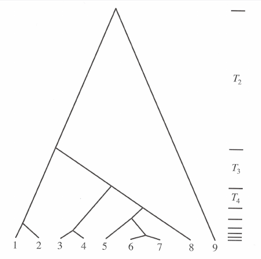
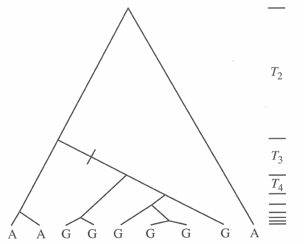
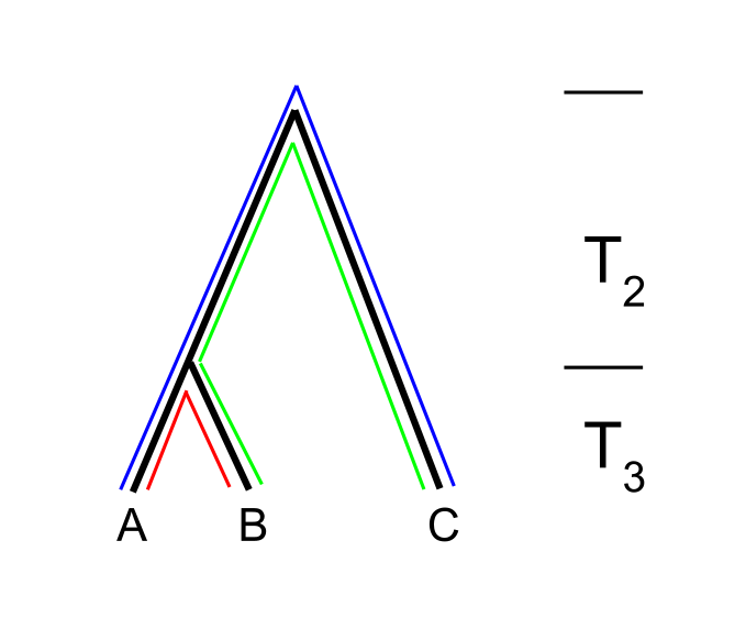
Let’s mark the coalescence time of \(i\) lineages with \(T_i\). Using units of \(N\) generations, for the next coalescence event
- expected value is \(E(T_{i}) = \frac{2}{i(i-1)}\)
- variance is \(\text{Var}(T_i) = (\frac{1}{i(i-1)})^2\)
With this we can compute the expected time for the next coalescence event for different values of \(i\):
| \(i\) | \(E(T_i)\) | \(\text{Var}(T_i)\) |
|---|---|---|
| 2 | 1 | 1 |
| 3 | 0.3333 | 0.1111 |
| 4 | 0.1667 | 0.0278 |
| 5 | 0.1 | 0.01 |
| 6 | 0.0667 | 0.0044 |
| 7 | 0.0476 | 0.0023 |
| 8 | 0.0357 | 0.0013 |
| 9 | 0.0278 | 0.0008 |
| 10 | 0.0222 | 0.0005 |
| 11 | 0.0182 | 0.0003 |
| 50 | 0.0008 | 0 |
| 100 | 0.0002 | 0 |
| 1000 | 0.000002 | 0 |
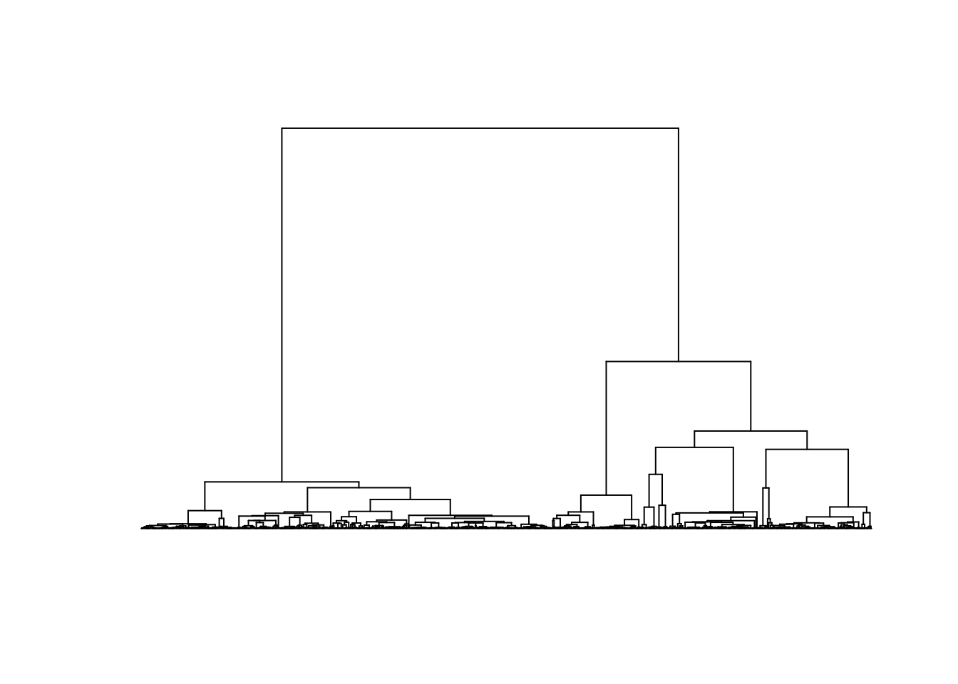
The consequences of this can be seen in examples of a coalescence tree for n=10 (left) and n=1000 (right):
The coalescence events happen quickly when \(i\) is large and the few last lineages take most of the time to join.
Simulating coalescence trees
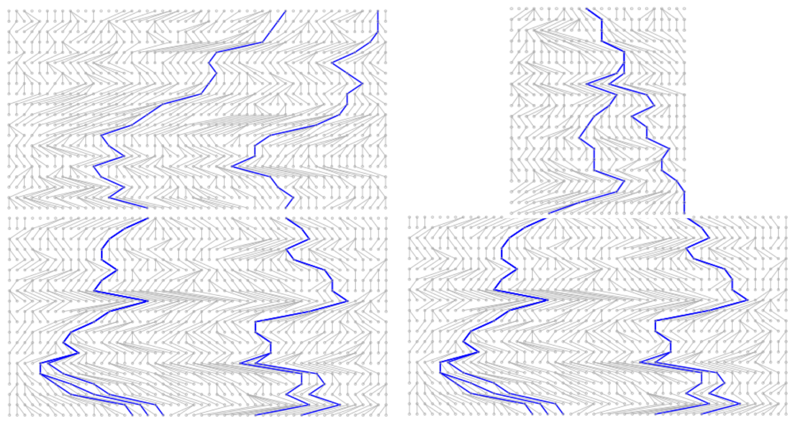
You can test how the shape of coalescence tree changes (or doesn’t change) depending on the number of lineages sampled. Below, nine coalescence trees are simulated for the number of sampled lineages provided.
- Try simulating trees with different numbers of sampled lineages and focus especially on the distribution of branch lengths on the y-axis. Think about the variance of branch lengths in different parts of the tree.
From the time to the next coalescence event, we can calculate the expected time for all lineages joining, i.e. the time to the most recent common ancestor \(T_{MRCA}\), and the total length of the coalescence tree, \(T_{total}\):
- expected time is \(E(T_{i}) = \frac{2}{i(i-1)}\)
- \(T_{MRCA} = \sum_{i=2}^nT_i = \sum_{i=2}^n\frac{2}{i(i-1)}=2(1-\frac{1}{n})\)
- \(T_{total} = \sum_{i=2}^niT_i = \sum_{i=2}^ni\frac{2}{i(i-1)}=2\sum_{i=1}^{n-1}\frac{1}{i}\)
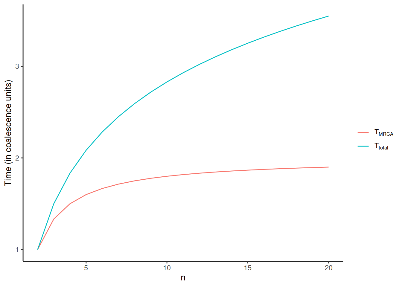
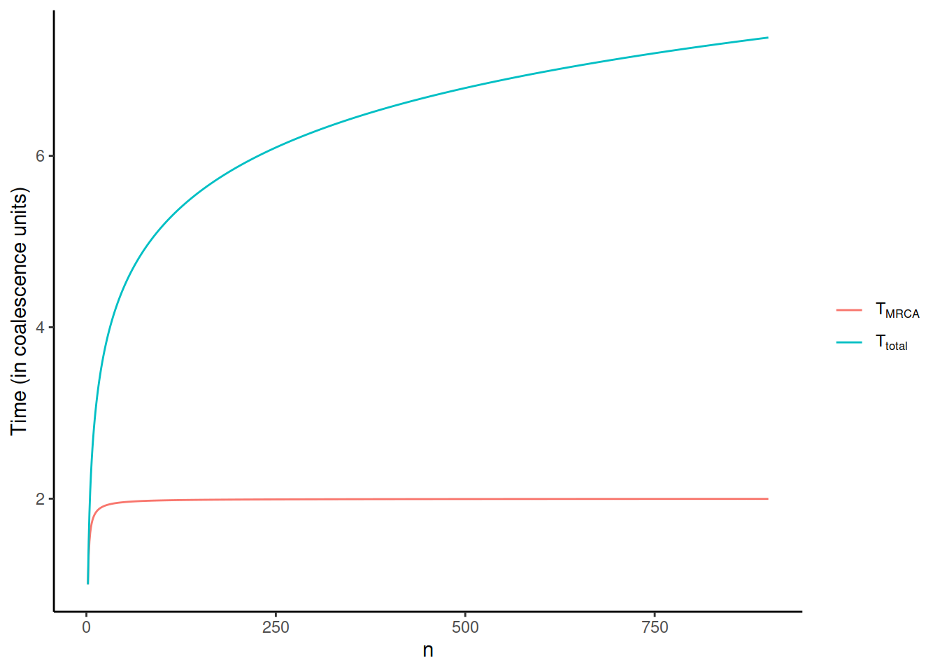
It is notable how these two functions behave when \(n\) increases:
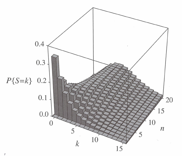
\(T_{total}\) keeps increasing, albeit more slowly, forever, whereas \(T_{MRCA}\) reaches 2 when \(n\) goes to infinity. On the other hand, \(T_{total}\) increases much faster in the very beginning and the growth after e.g. n=100 is modest. As seen below, this has consequences for the sampling of individuals for a study: \(T_{total}\), the total length of the coalescence tree, reflects the nucleotide diversity of the sample. In the beginning, the diversity increases rapidly with additional samples but, after a while, the line levels and adding new samples doesn’t bring much new variation.
Neutral genetic variation
The properties of coalescence process are of no great interest if all the sequences are identical. They can become non-identical through mutations. When discussing mutations here, we assume that they are neutral, never occur twice at the same position (infinite sites model) and the population considered is haploid.
We define
- the rate of mutations per site per generation is \(\mu\)
To give an idea of the size of \(\mu\), the estimates for humans vary between \(1 × 10^{-8}\) and \(3 × 10^{-8}\).
The number of mutations between two samples (or lineages) is such an important concept that it has a term of its own, \(\theta\). As we now know that the coalescence time for two samples is 1 (coalescence unit) and the mutations accumulate in both lineages:
we can define
- mutations between two lineages is \(\theta=2N\mu\)
- mutations per unit of time is \(\dfrac{\theta}{2}\)
Related concepts are
- \(S\) is the number of segregating (=variable) sites in the sample of N sequences
- \(\pi\) (pi) is the average number of differences between pairs of sequences
- \(\eta_i\) (eta) and \(\xi_i\) (xi) are the number of sites segregating at different frequencies in folded and unfolded allele frequency spectrum
We can derive the latter from the former.
Segregating sites
Given
- \(T_{total} = \sum_{i=2}^niT_i = \sum_{i=2}^ni\frac{2}{i(i-1)}=2\sum_{i=1}^{n-1}\frac{1}{i}\)
- \(\dfrac{\theta}{2}\) mutations per unit of time
the number of mutations in the whole tree is
\[E(S) = E(K)E(T_{total}) = (\frac{\theta}{2})(2\sum_{i=1}^{n-1}\frac{1}{i}) = \theta \sum_{i=1}^{n-1}\frac{1}{i}\]
Pairwise differences
Similarly for \(\pi\)
\[E(\pi) = \frac{1}{\binom n2} \sum_{i=1}^{n-1}\sum_{j=i+1}^{n}\frac{\theta}{2}E(2T_{ij}) = \frac{\theta}{\binom n2} \sum_{i=1}^{n-1}\sum_{j=i+1}^{n}E(T_{ij})\]
It can be shown that \(E(T_{ij})=1\) and thus \(E(\pi)=\theta\).
Site frequencies and site frequency spectra
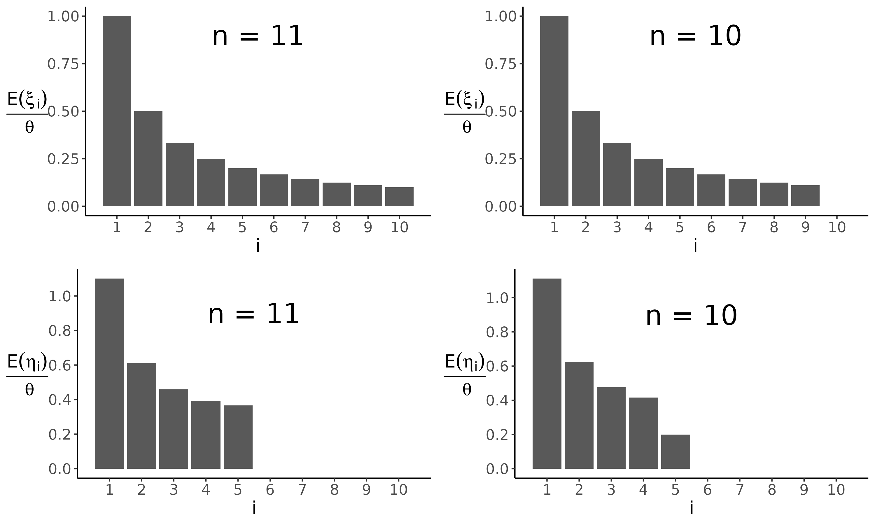
\(\xi_i\) is the number of segregating sites where the mutant base is present in \(i\) sequences and the ancestral base is present in all other \(n-i\) sequences
- \(\tau_i\) is the total length of branches that have \(i\) descendants in the sample
It can be shown that \(E(\tau_{i})=\frac{2}{i}\) and thus
\[E(\tau_i)=\frac{\theta}{2}E(\tau_i)=\frac{\theta}{i}\ \ \text{~for~} 1\leq i \leq n-1\]
When the ancestral base is not known, the number of derived alleles naturally cannot be determined; however, even in such cases, the frequency of the minor allele (less frequent allele) can be determined. Calculating MAFs is the same as folding the frequencies of derived alleles in the middle, i.e. combining the counts of sites where the derived allele is present in \(n-i\) sequences with those for \(i\) sequences. Although this may seem drastic, useful amounts of information are still retained.
- \(\eta_i\) (eta) is the number of segregating sites where the less frequent base is present in \(i\) sequences
\[ E(\eta_i) = \theta\frac{\frac{1}{i}+\frac{1}{n-i}}{1+d_{i,n-i}} \ \ \text{~for~} 1\leq i \leq (n/2)\]
where \(d_{i,j}=1 \ \text{~if~} i=j\) and \(d_{i,j}=0 \ \text{~if~} i\neq j\)
The difference between unfolded (top) and folded (bottom) distributions becomes clear when the number of chromosomes is even and thus the maximum number of segregating alleles is odd:
In the exercises, we will use unfolded site frequency spectra.
Coalescence in non-constant populations
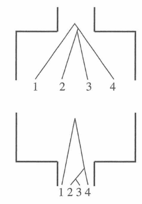
Coalescence rate is measured in units of N (haploid) or 2N (diploid) generations. Using these units, the expected times do not change between different-sized populations but the units of measurement may change: one unit means a greater number of generations in a large population than in a small population.
Assume a coalescence process with a constant population size
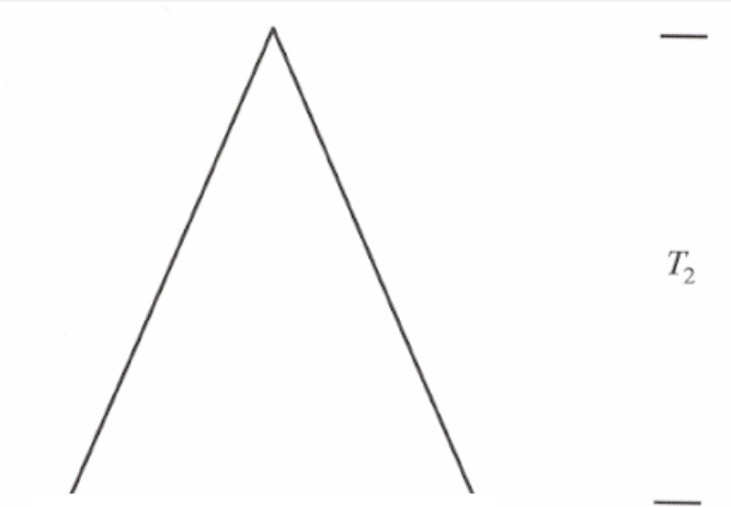
- at time \(t\) (the break in the figures below), two lineages remain
- expected time for coalescence is \(N\) generations
- if \(N\) is large (left), coalescence is slow
- if \(N\) is small (right), coalescence is rapid
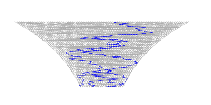
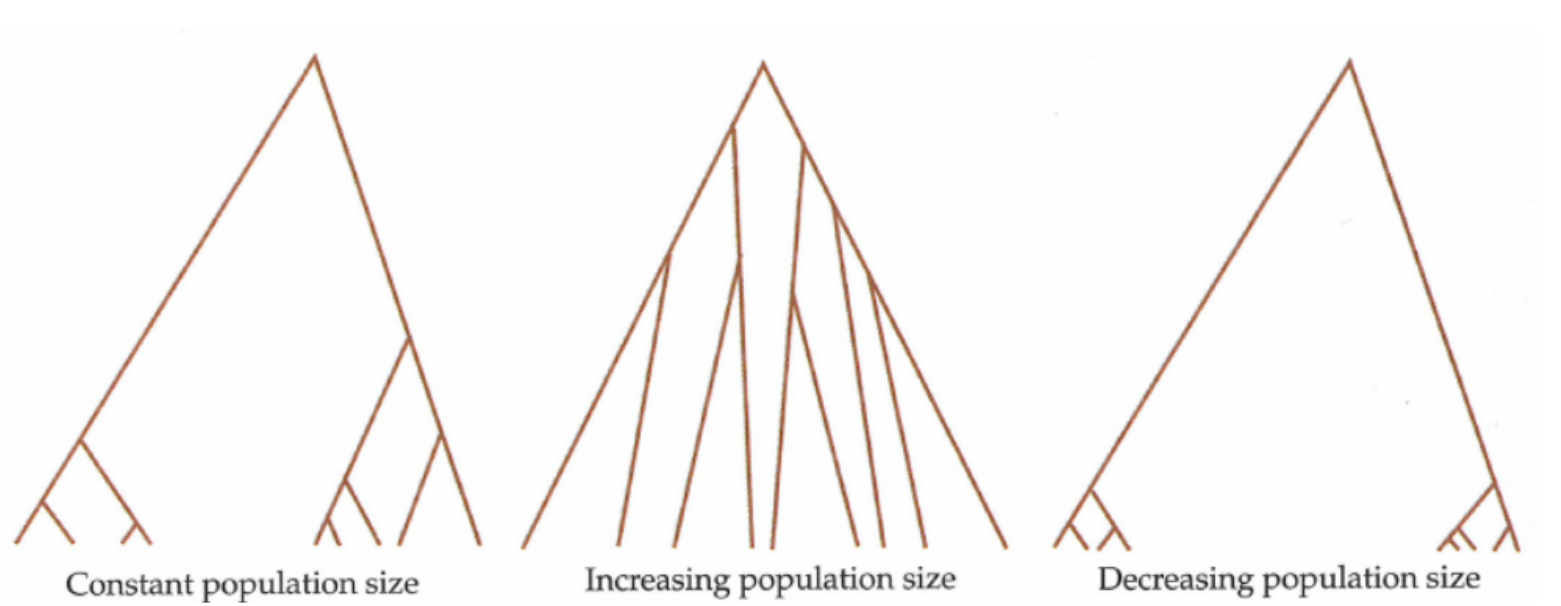
In practice, the change in population size is more gradual but the concept still holds. In population with a decreasing size, we expect many coalescent events to take place in the most recent past during the small population phase; lineages that survive the small population phase may then take long time to coalesce in the large population phase:
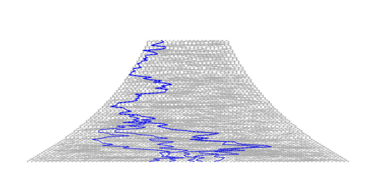
In population with a growing size, we expect few coalescent events to take place in the most recent past during the large population phase; lineages that survive the large population phase coalesce rapidly in the small population phase:
Tree shape and site frequency spectrum
Population demography, i.e. the changes in the population size, affects the expected tree shape. The mutation process is random: we can think mutations falling on the branches of the trees below and the probability of them hitting a particular branch depends on its length. Depending on the branch that the mutation hits, the newly derived allele will be inherited by different numbers of offspring. As a result, the tree shape affects expected site frequency spectrum.
Coalescence under migration
Migration means transfer of individuals between populations. If a lineage has moved between populations, this must affect its coalescence process with other lineages.
Migration increases the coalescence time but, rather surprisingly, the migration rate (\(m\)) has (in some cases) no impact. One way of thinking this is that \(m\) may affect the variance of the coalescence times but not their mean. If \(m\) is low, the two lineages are likely to stay in the same population until they coalescence and the time for that is short; however, if one of the lineages happens to migrate, it takes long time for the lineages to end up in the same population and the time for the coalescence is super long. If \(m\) is high, the two populations become practically one.
Let’s define
- \(m\) is the rate of migration per individual per generation
- \(M=Nm\) is the scaled migration rate (assuming small \(m\), large \(N\))
then, for \(n=2\) and two subpopulations of size \(N\) each, the expected coalescence time is
- \(E_S(t) = 2\) when the two lineages are sampled from the same subpopulation
- \(E_D(t) = \frac{1}{2M}+2\) when the two lineages are sampled from different subpopulations
Coalescence under subdivision
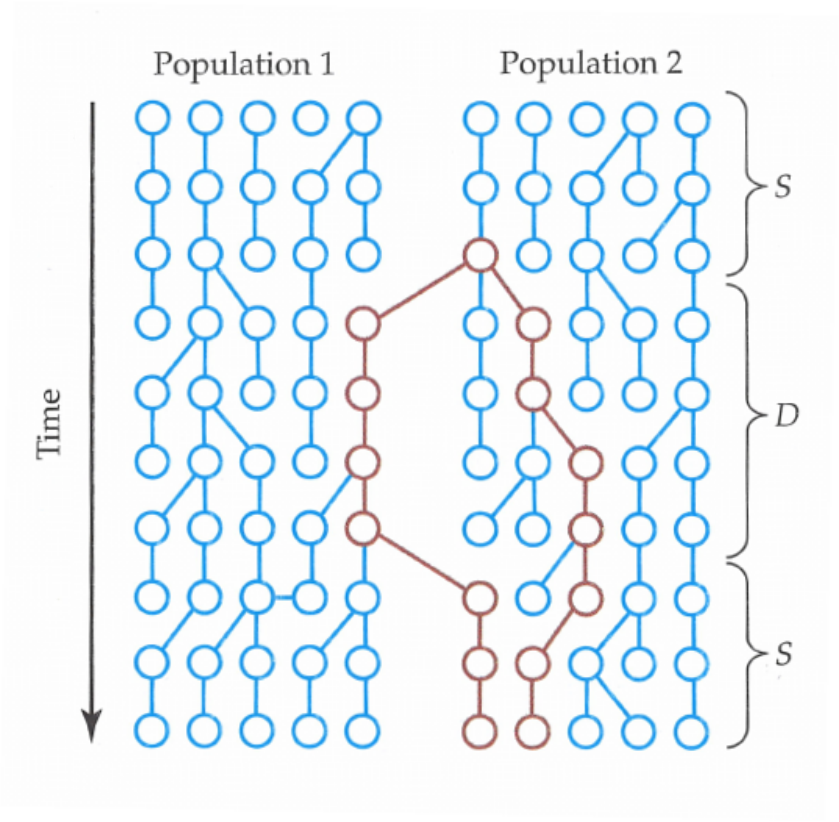
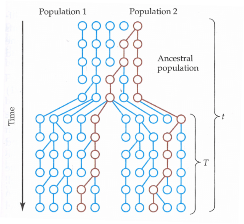
Populations may split and diverge without subsequent gene flow. Sometimes this population substructure is hidden and one may sample individuals without knowing that they belong to different subpopulations.
In the absence of migration, the expected coalescence times are simply:
- \(E_S(t) = 1\) when the two lineages are sampled from the same subpopulation
- \(E_D(t) = T + 1\) when the two lineages are sampled from different subpopulations
where \(T\) is the time to the split event (see the figure above).
Demographic events and summary statistics
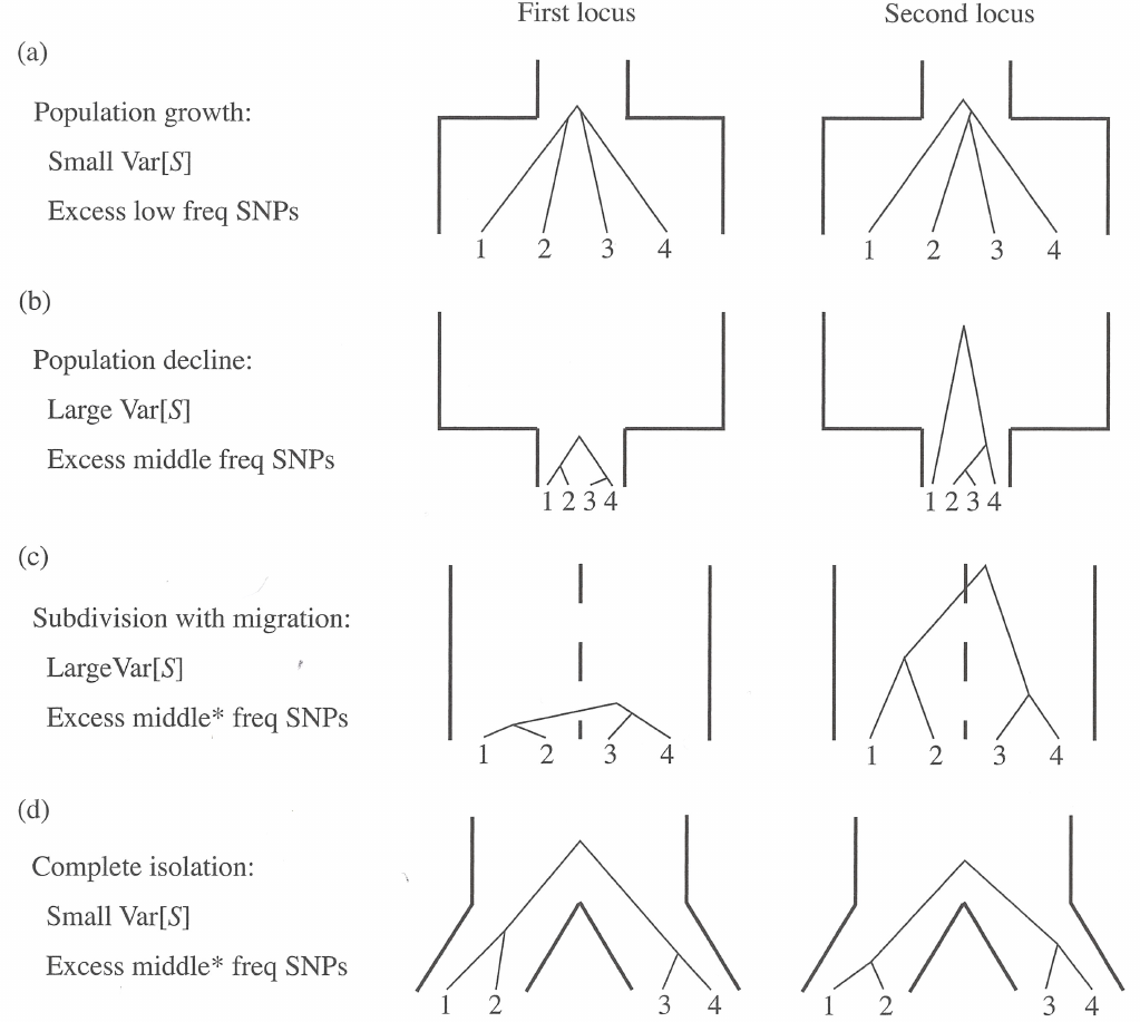
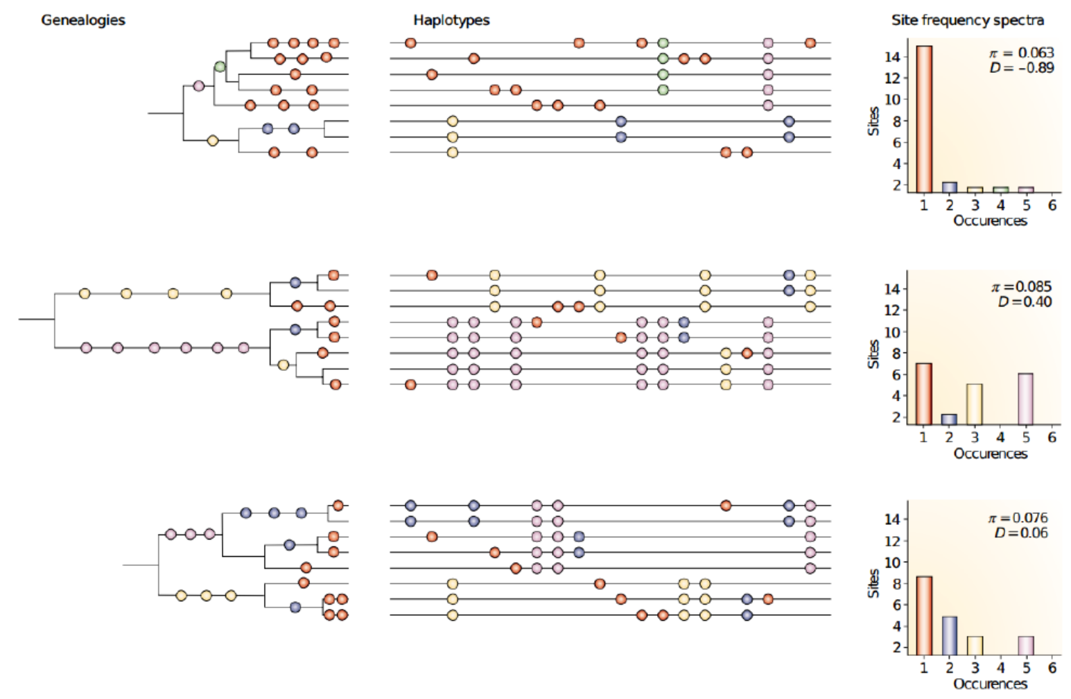
Different demographic events affect differently on common population genetic statistics. The figure below describes how different events affect on \(S\), the number of segregating sites, and site frequency spectrum (the number of alleles with different frequencies). The figure shows two loci (left and right) to illustrate that the patterns are either predictable (small variance across loci) or unpredictable (large variance across loci).
Tajima’s D
We saw earlier that \(\theta\) is involved in the equations to estimate \(S\), the number of segregating sites, and \(\pi\), the average pairwise differences between sequences:
- \(E(S) = \theta \sum_{i=1}^{n-1}\frac{1}{i}\)
- \(E(\pi) = \theta\)
These provide two estimators for \(\theta\), known as Watterson’s and Tajima’s estimators:
\[\begin{align*} \hat{\theta}_W &= S / \sum_{i=1}^{n-1}\frac{1}{i} \\ \hat{\theta}_T &= \frac{1}{\binom n2}\sum_{i=1}^{n-1}\sum_{j=i+1}^{n}k_{ij} \end{align*}\]
where \(k_{ij}\) is the number of differences between sequences \(i\) and \(j\).
If the population has evolved under the neutral WFM, the two estimators are in agreement and Tajima’s \(D = 0\):
\[ D = \frac{\theta_T-\theta_W}{\sqrt{\hat{V}(\theta_T-\theta_W)}}\]
If \(D>2\) or \(D<-2\), the standard neutral model is rejected. The reasons for rejections are many, including non-constant population size and selection.
Variants of Tajima’s \(D\) are e.g. Fu and Li’s \(D*\) and \(F*\) that consider also the number of singletons.
In general, all related test statistics are functions of the site frequency spectrum: as shown above, demographic history (and selection) affect the SFS. As an example, we can look at the schematic trees from the figure above:
If one thinks of mutations falling on these tree branches, it is easy to see where they cause singletons and where they are more likely inherited by multiple descendants. Then, one can reason how the singletons and non-singletons affect the two \(\theta\) estimators and what will be the value of Tajima’s \(D\).
Interpretation of Tajima’s D
Tajima’s D is a function of \(S\) and \(\pi\) and there can be many reasons for these two to differ. Typically, there’s always a demographic explanation (changes in population size) and a selection pattern giving a similar footprint:
| Value of Tajima’s D | Biological interpretation 1 | Biological interpretation 2 |
|---|---|---|
| Tajima’s D=0 | Observed variation similar to expected variation | Population evolving as per mutation-drift equilibrium. No evidence of selection |
| Tajima’s D<0 | Rare alleles abundant (excess of rare alleles) | Recent selective sweep, population expansion after a recent bottleneck, linkage to a swept gene |
| Tajima’s D>0 | Rare alleles scarce (lack of rare alleles) | Balancing selection, sudden population contraction |
(See Wikipedia for more details.)
In the figure below, the top row has \(D<0\) and this could be caused by a recent population growth, the locus being under positive selection (new variants are favoured) or a recent selective sweep having wiped out previous variation. The second row has \(D>0\) and this could be caused by a recent population decline or the locus being under balancing selection and thus retaining very old haplotypes. The bottom row has \(D\sim0\) as would be expected under neutral evolution.
Site frequency spectra as input for downstream analyses
The site frequency spectra, also known as site allele frequencies (SAF) or derived allele frequencies (DAF), are a powerful summary data for downstream inferences. These inferences vary from selection studies to demographic inferences.
Above, we saw that the SAF distribution is given by:
\[E(\tau_i)=\frac{\theta}{2}E(\tau_i)=\frac{\theta}{i}\ \ \text{~for~} 1\leq i \leq n-1\]
However, this assumed that the sites are 1) evolving neutrally (no selection) and 2) the population size is constant.
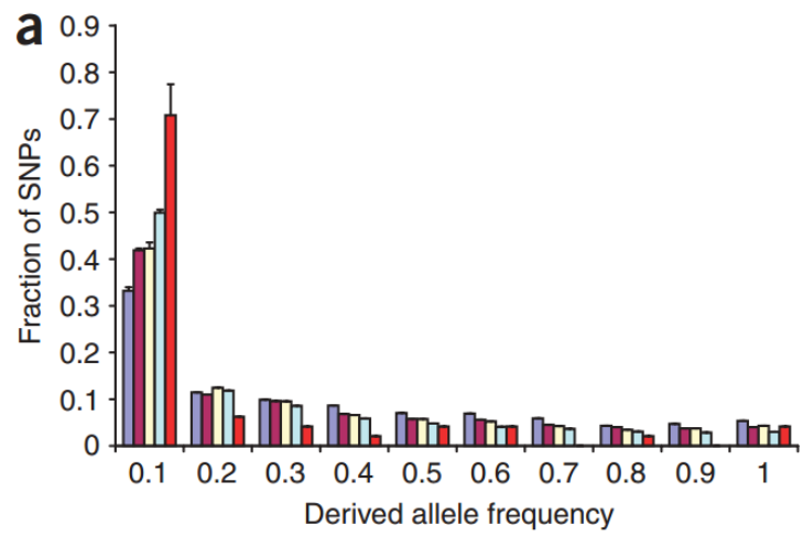
The coalescent theory applies only for neutrally evolving sites. Using other methods, it can be shown that the distribution differs from the expectation if the sites are under negative selection. The figure below shows the SAF distribution for conserved miRNA sites (in red) and various other site categories (from Chen and Rajewsky, 2006):
The conserved miRNA sites are highly enriched in the lowest frequency category, suggesting that the negative selection is removing derived alleles in those sites and pushing the frequencies towards left.
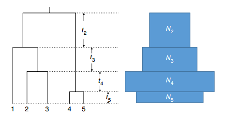
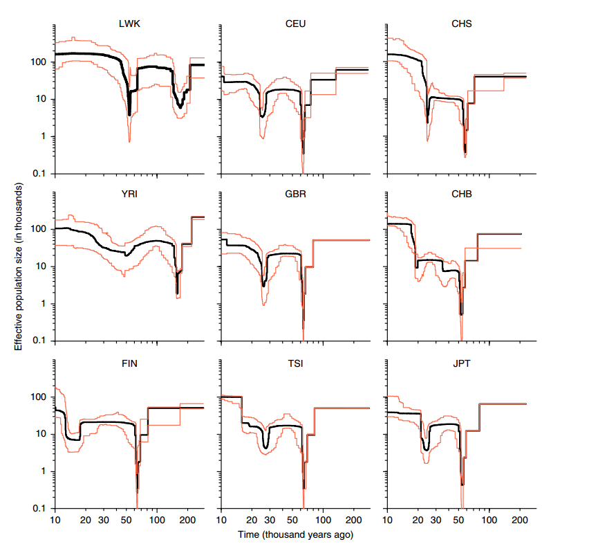
Other kinds of deviations are seen when the sites are evolving neutrally but the population size is not constant. There are many methods trying to fit a demographic model that would produce the observed SAF. One of them is Stairway plot that models the history as time segments such that the population size is constant within a segment but can change between the segments:
Using this approach, they showed that the non-African human populations share a population bottleneck around 65 kya that the African populations do not have:
They also noted that the ancestors of the Finns potentially experienced a recent bottleneck between 10,000 and 20,000 years ago.
Much of the mathematics is beyond the level of this course and is omitted. There are some concepts that important to understand.
The coalescence process is a random process and the shape of coalescence tree can vary greatly and, especially for for small \(n\), the variance of the expected times can be large. Nevertheless, the tree has a characteristic outlook of many short terminal branches (the first lineages coalesce rapidly) and a few very long internal (or terminal) branches (the last lineages coalesce very slowly).
Due to recombination, the coalescence tree varies across the genome and the “average tree” estimated from genome data doesn’t show the same shape. However, the time to MRCA still reflects the population size \(N\) and MRCA of a small population is much closer in time than that of a large population.
\(T_{MRCA}\) and \(T_{total}\) are quite straightforward to derive from the coalescence theory. It is important to understand their difference and relation to the expected genetic diversity and the number of segregating sites when \(n\), the number of sampled sequences, increases.
It may feel surprising that the expected values of \(\pi\) (nucleotide diversity in a sample of many individuals) and \(H\) (heterozygosity of a diploid individual from that sample) are identical, though the variance for the latter is much greater. On the other hand, \(\pi\) reflects the number of differences between two chromosomes drawn randomly from a population whereas \(H\) reflects the number of differences between the chromosomes inherited from a mother and a father, supposedly drawn randomly from a population.
The expected shape of an unfolded site frequency spectrum of neutral derived alleles is given by \(\frac{\theta}{i}\). There are many reasons why the distribution deviates from this but the expected shape – including the high number of singletons, i.e. derived alleles observed exactly once – is important for comparisons.

