flowchart LR
    subgraph sample_1
    style sample_1 fill:#fdf2e9
    fastq_1[" fastq_1 "] --> bam_1[" bam_1 "]
    bam_1 --> gvcf_1[" gvcf_1 "]
    end
    subgraph sample_2
    style sample_2 fill:#fdf2e9
    fastq_2[" fastq_2 "] --> bam_2[" bam_2 "]
    bam_2 --> gvcf_2[" gvcf_2 "]
    end
    subgraph sample_n
    style sample_n fill:#fdf2e9
    fastq_n[" fastq_n "] --> bam_n[" bam_n "]
    bam_n --> gvcf_n[" gvcf_n "]
    end
    subgraph sample_100
    style sample_100 fill:#fdf2e9
    fastq_100 --> bam_100
    bam_100 --> gvcf_100
    end

    gvcf_1 --> gvcf
    gvcf_2 --> gvcf
    gvcf_n --> gvcf
    gvcf_100 --> gvcf

    subgraph all_samples
    style all_samples fill:#fdf2e9
    gvcf --> vcf
    end
2. Short reads and their mapping
After this chapter, the students can describe the technology behind short-read DNA sequencing and list the main steps in the computational processing of short-read data. They can also explain the concept “sequencing depth” and the stochastic process that affects its variation across the genome sites.
Quality of the reference genome affects the analyses based on it, but the seriousness of the impact depends on the specific analysis. Many population genetic analyses are surprisingly insensitive to the continuity (or fragmentation) of the reference genome while others require long intact stretches of the genome to work properly. Some properties of genomes impact downstream in a similar manner in the case of good continuous and poor fragmented reference genomes. The impact of the reference genome starts in the very beginning, in the short-read read mapping.
Our workflow
Our workflow for variant calling is the following:
In this, the first step from FASTQ to BAM is called “read mapping” or “read alignment”.
Short-read sequencing
The most affordable approach for whole genome sequencing (WGS) is so called short-read sequencing and it is thus widely used in WGS-based population genetic studies. The field was long dominated by company Illumina (using technology developed by Solexa) and the short-read sequencing is commonly called “Illumina sequencing”. New variations of the approach have been introduced by Element Biosciences (AVITI platform) and BGI (BGISEQ platform).
The approach is explained well in many YouTube videos such as this:
In brief, the Illumina approach is the following:
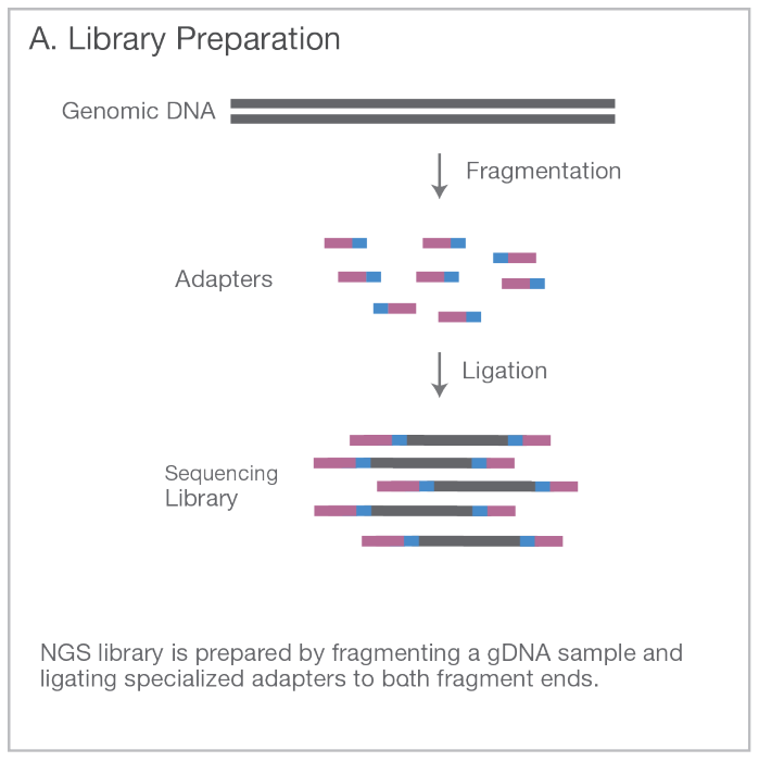
Break the full genome (WGS) DNA into small fragments. Select fragments around ~300 bases in length. Add adapters to the end of the fragments.
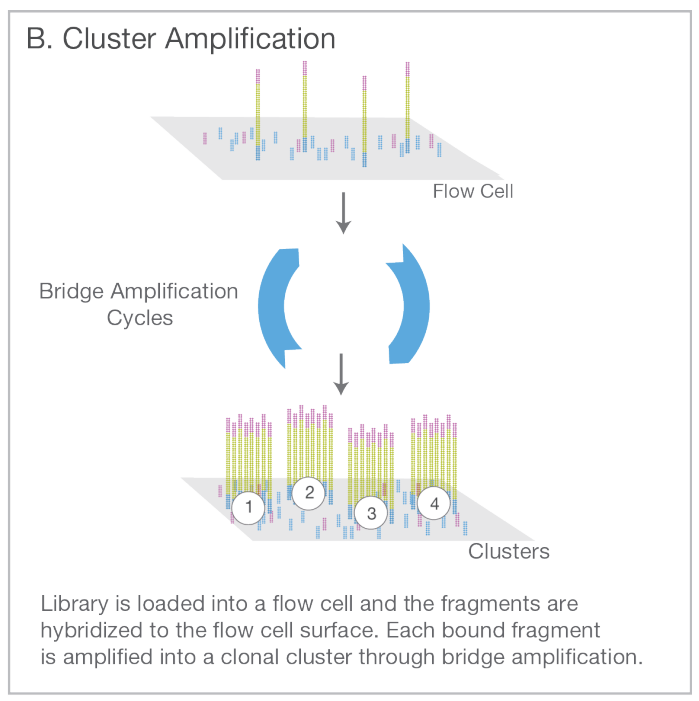
Attach the fragments on a slide with a lawn of surface-bound oligos complementary to the adapters. Amplify the fragments with PCR creating a cluster of identical sequences.
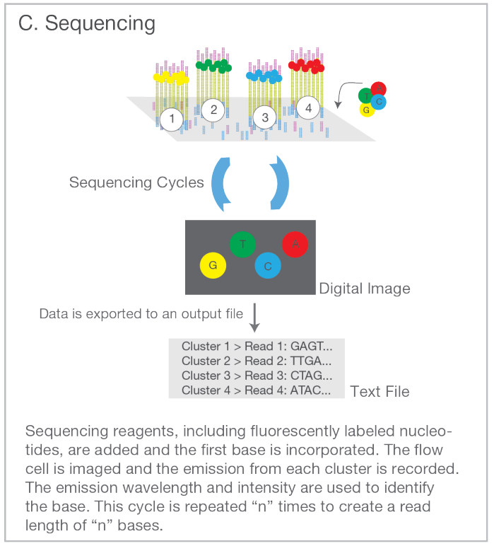
Sequence each fragment cluster by adding nucleotide molecules with a colour tag attached to them. On each round, take an image of the slide: the millions of small dots represent the distinct clusters, each originating from one genomic fragment; the colour of the dot indicates the type of the latest base. After reading one end of the fragment, attach the other end to the slide (shown in pink) and release the original end (shown in blue). Repeat the sequencing steps.
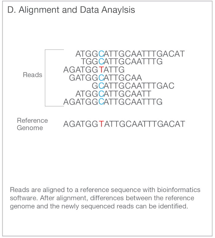
Map the reads to the reference genome. With sufficiently large numbers of reads, each genome position is covered by multiple overlapping fragments and the bases in both copies (maternal and paternal) of the genome can be identified.
A common practise is to sequence 150+150 bp pair-end reads, that is to resolve 150 bp from both ends of the fragment either leaving a short unknown spacer between them or the reads slightly overlapping in the middle. Assuming that the studied sample and the reference genome are largely similar, the two reads are placed close to each other at the opposite strands of the reference genome with their heads pointing inwards. If that is not the case, one or both of the reads are incorrectly mapped or the sample and the reference differ from each other e.g. by structural change (translocation, inversion etc.)
Read mapping
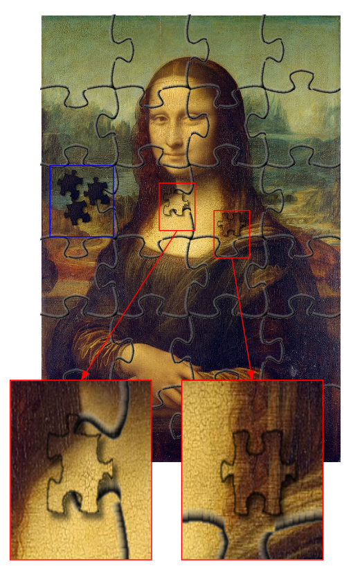
In the previous section about reference genomes, one could see two images of Mona Lisa: one was made of large pieces and complete while the other was made of small pieces and lacked the difficult, highly repetitive and non-unique, regions. If we had multiple similar portraits of ladies and our aim was to identify the persons and see the differences between them, one could argue that the two images would do roughly equally well. The parts missing from one of the images are uninformative for analyses trying to understand the differences between multiple images; even if using the more complete version of the image, one could consider ignoring them as they may produce unknown errors and biases. The true information is in the unique bits and those even the less complete version has got right.
This is very much the situation in population genetic analyses. Genomes are huge and they typically contain sufficient information for most population genetic analyses even after removal of a significant proportion of the data. Moreover, population genetic methods are typically built on simple base substitution models (and the coalescent theory) and even if the data over the repetitive regions were perfectly correct, the evolution of those regions could violate the assumption of the model (e.g. due to gene conversion, replication slippage etc.) and introduce error in the analysis. As a result, many population genetic analyses can be performed fairly well even with fragmented reference genomes as long as it approximately haploid and doesn’t contain too many erroneously duplicated regions. Of course, a more continuous reference improves some analyses and should be utilised if available.
Placement – or mapping – of reads to a reference genome is straightforward, similar to finding the places of small jigsaw pieces on a copy of the same image. The computational methods for read mapping are highly advanced and utilise an index of the reference that allows quickly excluding the possible places for the read. (See “Burrows-Wheeler Transform” below if you are interested in going to details.)
In our analyses, we won’t worry too much about the placement of reads from non-unique sequence regions and, in most cases, remove them from the data even if they were possibly correctly placed.
We map our short-read data with the program bwa mem (github.com). The program minimap2 (github.com) is a new alternative for bwa mem and superior in the alignment of very long sequences (it can align two full genomes in a few minutes!). In the alignment of classical short-read data, the two methods should be comparable and, on this course, we use the older and still more widely used bwa mem.
The name bwa stands for “Burrows-Wheeler Aligner” which comes from the computer science concept “Burrows-Wheeler Transform”. The theoretical background of read mapping is explained in the excellent introduction to suffix arrays, BWT and FM index by Alan Medlar:
Sequence reads
FASTQ
Short-read sequencing data are provided in FASTQ format (Wikipedia) that consists of a header line, a sequence line and a base-call quality line, shown below in red, blue and magenta, respectively. (In between the last two, there is now unused line for comments.) Typically, the reads are provided in two files such that the forward and backward read from each fragment are provided in the same order. One file may consist of millions of reads, each read consisting of four lines.
A typical read could look like this:
@K00137:79:H3KNNBBXX:3:1101:1030:21850
TTTGACCATTATTGTTACTTTTAAAGCTTTTGCAGAAGGAGTAAACAGCTAAAACAGAATGTATGAAGAAGGCTTTAGCTTACACTGTTTCTATCAAGCAAATGACCTTTTTTAATCATTA
+
AAFFFKKKKKKKKKKKKKKKKKKKKKKAKKKKKKAKKK7FKKKKKKKKKKKKKKKKKKKFKKKKKKKFKFAFFKKKKKAFKKKKFKKKKKK<FKFKKKKKKKAAKK<AKKK,,,,,,,,A,
If we break up the header line “K00137:79:H3KNNBBXX:3:1101:1030:21850” into pieces, the different parts indicate this:
- K00137: unique instrimunt name
- 79: run id
- H3KNNBBXX: flowcell id
- 3: flowcell lane
- 1101: tile within the flowcell lane
- 1030: x-coordinate of the cluster (dot) within the lane
- 21850 y-coordinate of the cluster (dot) within the lane
Moreover, we can use the information here to learn that “H3KNNBBXX” was “(8-lane) v1 flow cell” on a Illumina HiSeq 4000 device.
Although compressions of unmapped reads doesn’t reduce the size of the file very much (if you wonder why, you can search for a tutorial of compression such as one here), it is highly recommended to compress the data. The downstream applications can fluently handle gzip-files.
The reads are aligned – or mapped – to a reference genome; the output of that is provided in SAM/BAM format that retains everything from the FASTQ and adds information about the mapping.
SAM/BAM
When the read above is mapped, it is converted SAM/BAM format (Wikipedia) may look like this:
K00137:79:H3KNNBBXX:3:1101:1030:21850 163 ctg7180000008138 10224 0 150M = 10362 288 TTTGACCATTATTGTTACTTTTAAAGCTTTTGCAGAAGGAGTAAACAGCTAAAACAGAATGTATGAAGAAGGCTTTAGCTTACACTGTTTCTATCAAGCAAATGACCTTTTTTAATCATTA AAFFFKKKKKKKKKKKKKKKKKKKKKKAKKKKKKAKKK7FKKKKKKKKKKKKKKKKKKKFKKKKKKKFKFAFFKKKKKAFKKKKFKKKKKK<FKFKKKKKKKAAKK<AKKK,,,,,,,,A, NM:i:5 MD:Z:113C7T0C16T4T5 AS:i:125 XS:i:125 RG:Z:sample-1
The header line (QNAME), the sequence line (SEQ) and the base-call quality line (QUAL) have not changed. The remaining fields are:
| # | Field | Meaning |
|---|---|---|
| 1 | QNAME | Query template/pair NAME |
| 2 | FLAG | bitwise FLAG |
| 3 | RNAME | Reference sequence NAME |
| 4 | POS | 1-based leftmost POSition/coordinate of clipped sequence |
| 5 | MAPQ | MAPping Quality (Phred-scaled) |
| 6 | CIGAR | extended CIGAR string |
| 7 | MRNM | Mate Reference sequence NaMe (`=’ if same as RNAME) |
| 8 | MPOS | 1-based Mate POSition |
| 9 | TLEN | inferred Template LENgth (insert size) |
| 10 | SEQ | query SEQuence on the same strand as the reference |
| 11 | QUAL | query QUALity (ASCII-33 gives the Phred base quality) |
| 12+ | OPT | variable OPTional fields in the format TAG:VTYPE:VALUE |
The SAM format specification is provided at https://samtools.github.io/hts-specs/SAMv1.pdf.
In a FLAG (explained on page 7 of the format specs), the zeros and ones can be seen as switches – ON vs OFF – such that the combination of switches makes the full binary number. (Binary numbers are explained on EEB-021.) For practical reasons, this binary number is converted to a decimal number in the samtools command.
A useful tool to play with flags is at https://broadinstitute.github.io/picard/explain-flags.html. Check what “163” means.
RNAME and POS are quite obvious, the chromosome (or contig) and the position within that where the read is mapped. MAPQ is the quality of that mapping: it is zero if there are multiple equally good places for the read. MRNM
MRNM, MPOS and TLEN are related to the pair of this read: if this is the orange read in the figure below, these specify the mapping position of the blue read (left) and the inferred length of the fragment (right).
The information on whether the read in question is the forward read (orange) or the backward read (blue) is given in the FLAG (“reverse strand”).
The read sequence (SEQ) was given in SAM/BAM exactly as in FASTQ. What if the read doesn’t match perfectly to the reference but contains insertions or deletions? That information is given by the CIGAR field (see Wikipedia).
The CIGAR field consists of letter-number pairs where the letter is the alignment act and the number defines how many positions it applies to. The letters are the following:
| CIGAR Code | Description | Consumes query | Consumes reference |
|---|---|---|---|
| M | alignment match (can be a sequence match or mismatch) | yes | yes |
| I | insertion to the reference | yes | no |
| D | deletion from the reference | no | yes |
| S | soft clipping (clipped sequences present in SEQ) | yes | no |
| H | hard clipping (clipped sequences NOT present in SEQ) | no | no |
| = | sequence match | yes | yes |
| X | sequence mismatch | yes | yes |
M, I and D refer to “match”, “insertion” and “deletion” and are the most commly seen. On should note that “match” means “not an indel” and can be between two non-identical bases.
For example, if we have the sequences ACGTAGAATA and ACTGCAGTA the alignment:
AC-GTAGAATA
ACTGCAG--TA
is specified as 2M1I4M2D2M. In our example SAM line above, the CIGAR string was 150M meaning that the full read was matches without indels.
In the CIGAR string, soft-clipping means that a part of the read sequence, which is shown in full, is not included in the alignment. One reason for that could be the low sequence quality towards the end of the read and the mapping algorithm deciding that the sequence is incorrect and unalignable. We’ll see later that this is not unproblematic. Hard-clipping is different and can be caused by first part of a read mapping to one chromosome and the second part to another chromosome. The read is then divided into two and the clipped sequence is not shown on this SAM line.
We use bwa mem for mapping and it doesn’t indicate if the matched bases in the read are identical to the reference or different. This information is not needed in the variant calling where it is only necessary to get the possible indels right and have the overlapping reads correctly placed. Some methods allow including the information about sequence identity in the CIGAR string using letters = and X.
Phred scores
In FASTQ, SAM/BAM and VCF formats, the quality scores are given using the Phred scale. The conversion of probability \(P\) to Phred score \(Q\) and back is done as
\[\begin{align*} Q&=-10~ log_{10}(P)\\ P&=10^{(Q/-10)} \end{align*}\]
If the sequencing machine reports the probability of a base at particular position of the read being wrong to be 10% (Perr=0.1), this gives log10(Perr)=-1 and Q=10. However, in the FASTQ/SAM files, there is only room for one character per base – the sequence line and the quality line have to be equally long.
The solution is to convert the numbers, rounded to integers, into letters. The range of Illumina quality scores for the accuracy of base call (“if we say that the base is ‘T’, what is the likelihood that it is not ‘T’ but something else”) is from 0 to 41, referring to probabilities 1 and 0.000079. The integer numbers are converted to ASCII characters (https://en.wikipedia.org/wiki/ASCII) but, as there are only 10 numbers, also non-numeric characters are used. In the ASCII table, the first characters are control characters (such as newline and TAB) and thus unsuitable; the 32nd character is space ’ ’ and still confusing. From 33 on, the characters are “printable”.
This gives the scale !-J (top row) to represent the Phred scores 0-41 (bottom row).
!"#$%&'()*+,-./0123456789:;<=>?@ABCDEFGHIJ
|                                        |
0.......................................41
Typically, Phred scores >=20 (probability of base being erroneous <=1%) is considered “good”.
A table showing selected Perr values and the corresponding log10(Perr), Q score and ASCII symbol.
| Perr | log10(Perr) | Q | symbol |
|---|---|---|---|
| 1 | 0 | 0 | ! |
| 0.1 | -1 | 10 | + |
| 0.01 | -2 | 20 | 5 |
| 0.001 | -3 | 30 | ? |
| 0.0001 | -4 | 40 | I |
Sequencing coverage
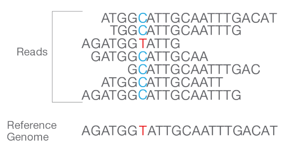
The schematic figure shown above contains and interesting detail:
There are seven overlapping reads that are otherwise in agreement but differ at one position, shown in blue and red. Six reads show that this position has C while one read indicates that it is T. The accuracy of experimental analyses is never 100% and how can we know if that T is true observation or a sequencing error? In this case, the row below shows that the reference has T at that position and thus T in the sample is highly likely correct and the individual is heterozygous, having T/C at that site.
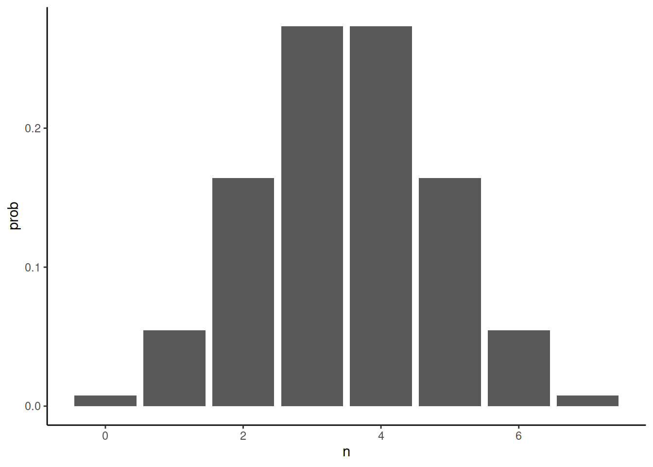
How likely is it that this would happen in reality? In sequencing experiments, one typically has lots of DNA and only a tiny proportion gets analysed. If the individual is heterozygous, 50% of the reads overlapping that site should have C and 50% should have T. The reads getting sequenced are assumed to be random sample with a 50% chance of drawing T at any time. The probability of getting n copies of T when sampling seven reads is given by binomial distribution. With R, it can be computed like this:
library(ggplot2)
ggplot(data.frame(n=0:7,prob=dbinom(x = 0:7, size = 7, prob = 0.5))) + geom_col(aes(n,prob)) + theme_classic()The probability of observing just on T is fairly small, 5.47%, and the probability of six Ts (and only one C) is the same. The probability of observing no Ts among seven reads when the individual is truly heterozygous is 0.78%. That sounds small but genome data may contain millions of variable sites and the probability of error would accumulate over these sites. For one million heterozygous sites all covered by seven reads, 15,625 could be expected to be erroneously inferred as homozygous (1e6 x 0.0078125 x 2)!
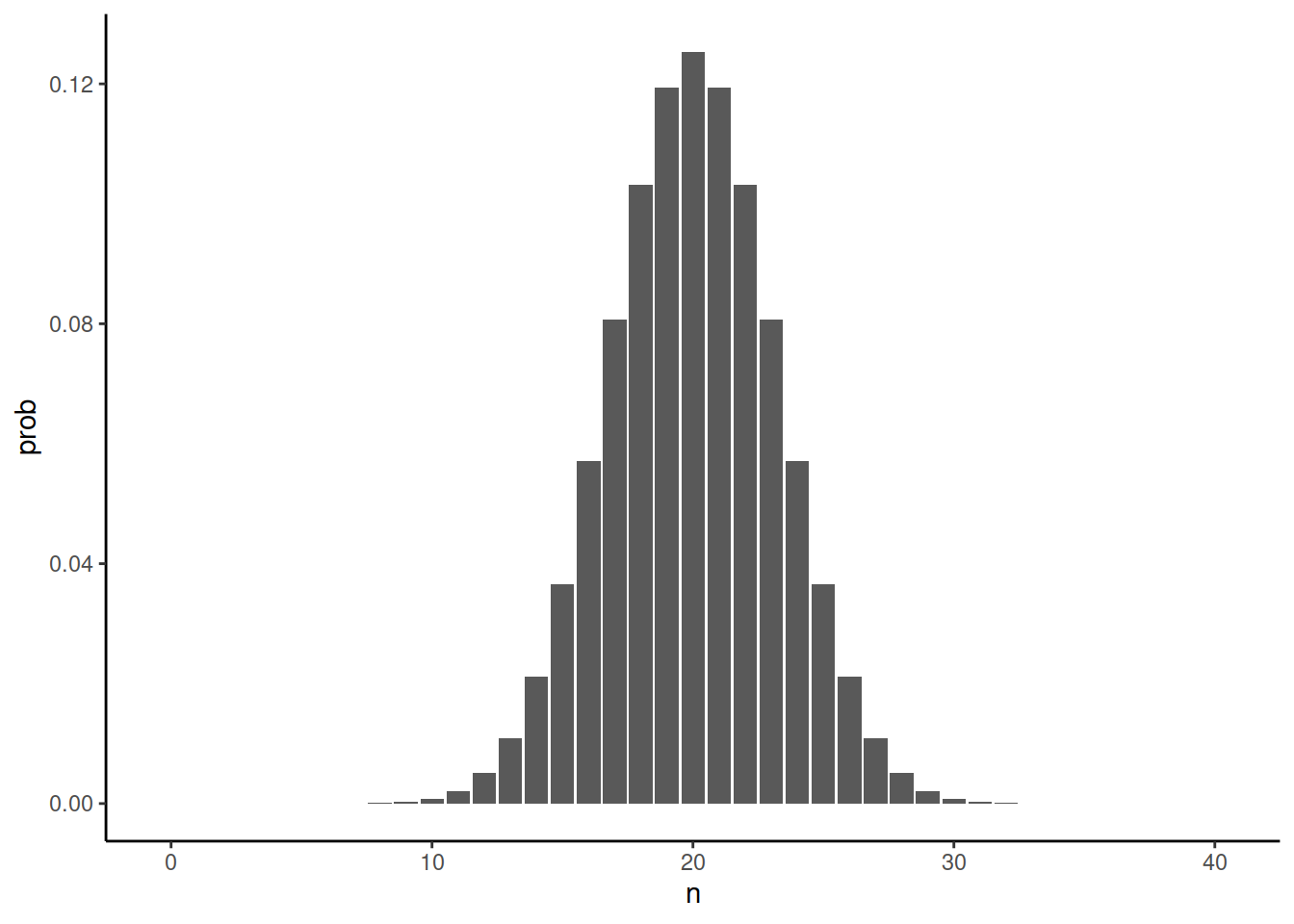
Is that bad? Yes and no. Ideally, one would like to have perfect data. In DNA sequencing, the quality of variant detection would be improved by sequencing more reads and thus covering each sites by more observations. The binomial distribution for 40 reads looks like this:
library(ggplot2)
ggplot(data.frame(n=0:40,prob=dbinom(x = 0:40, size = 40, prob = 0.5))) + geom_col(aes(n,prob)) + theme_classic()We can see that it is extremely unlikely not to observe both alleles at heterozygous positions. To be more precise, the chance is around one in a million. In fact, the probability of observing of observing either of the alleles less than five times across one million heterozygous sites is around one fifth:
p <- dbinom(0:40,40,0.5)
p[1]*2*1e6
[1] 1.818989e-06sum(p[1:5])*2*1e6[1] 0.1857024So why wouldn’t everyone want such high-coverage data? Because it costs money. There’s a small-ish fixed cost for making the sequencing library from each sample and much larger cost for producing sequencing data. When sequencing, one can mix the samples (called “multiplexing”) and reidentify the reads after the sequencing run (“de-multiplexing”). As a result, the sequencing coverage per sample can be easily adjusted and the cost per sample increases approximately linearly with the coverage. At the cost of sequencing one sample at 40x, one can sequence four samples at 10x or eight samples at 5x. In some analyses the accuracy is paramount but in population genetics, it is often more important to have a sufficient number of samples.
A second reason is that, in population genetics, heterozygosity of individuals is often less important than population-level allele frequencies, and the variance of the allele frequency estimates decreases with the number of samples. Moreover, at a locus with C and T alleles, one heterozygous individual may be incorrectly inferred as homozygous for C but then equally likely, another heterozygous individual be incorrectly inferred as homozygous for T. The two errors cancel out and the population-level frequencies of C and T are correct.
Short-read sequencing data are provided in FASTQ format that consists of a header line, a sequence line and a base-call quality line. The reads are mapped to a reference genome; the output of that is provided in SAM/BAM format that retains everything from the FASTQ and adds information about the mapping. The probability values are typically converted to Phred scores that can be further converted to ASCII characters. This saves lots of space without significant loss in accuracy.
DNA sequencing costs money and one has to balance between the accuracy of variant detection in individual samples and the number of individuals included in the analysis. In population genetic analyses, the accuracy of individual samples is not as important as the good sampling of multiple populations is often more important. On this course, we mostly analyse data sequenced at the coverage of 10x.
