2. Data processing from FASTQ to GVCF
After this practical, the students recognise FASTQ, BAM, GVCF and VCF data formats and can explain their roles and relationships. They can map FASTQ data to a reference genome using bwa mem and manipulate the resulting BAM data with samtools; and can call variants with GATK package using the joint-calling approach.
Getting to Puhti
Get to your working directory:
$ WORK=/scratch/project_2000598
$ cd $WORK/$USER
If you are on a login node (if you access Puhti through a stand-alone terminal, you get to a login node; in the web interface, you can select either a login node or a compute node), start an interactive job (see sinteractive -h for the options):
$ # the command below is optional, see the text!
$ sinteractive -A project_2000598 -p small -c 2 -m 4000 -t 8:00:00
These practicals contain relatively heavy computation the work should be done on a compute node or using SLURM jobs.
Preparations for the analyses
We have previously done the FASTA-index for our reference genome (reference/ninespine_rm.fa.fai) and will now generate a FASTA-dictionary:
$ module load samtools
$ samtools dict reference/ninespine_rm.fa > reference/ninespine_rm.dict
The dictionary will later be included in the VCF file.
The role of the dictionary is to provide a means to confirm that the VCF file (where it is integrated) and the external reference genome match. Without a dictionary, it would be possible that the VCF data were analysed against an incorrect reference and the results would therefore be wrong.
So, how to verify that the sequences are the same without writing the sequences? There are multiple versions of the human reference genome and each has chromosome names “chr1”, “chr2” etc. and the names are clearly not informative. The chromosome lengths would be better but, in theory, it is possible that a revision of the reference genome would remove sequence somewhere and add elsewhere, and produce an equally long but different sequence. The same length of two sequences does not mean that they are the same.
The start of the dictionary looks like this:
$ head -3 reference/ninespine_rm.dict @HD VN:1.0 SO:unsorted
@SQ SN:ctg7180000005484 LN:697083 M5:530cf96b9ecf6c85885876fa01820b82 UR:file:///scratch/project_2000598/$USER/reference/ninespine_rm.fa
@SQ SN:ctg7180000005545 LN:816998 M5:785bd5fdfe0aaf255c50a930e9c4cdba UR:file:///scratch/project_2000598/$USER/reference/ninespine_rm.faThe key is the field starting with “M5:”. This combination of commands produces the M5 string for the first contig:
$ samtools faidx reference/ninespine_rm.fa ctg7180000005484 \
  | grep -v ">" | tr -d '\n' | tr [acgtn] [ACGTN] | md5sum
530cf96b9ecf6c85885876fa01820b82 -The hash sum is the first part of the output. The second part - indicates that the sum was computed for STDIN. You can compare the output to that of:
$ md5sum reference/ninespine_rm.fa.faiNow, the sum and the target are clear.
Think about the commands and what they do. md5sum and cryptographic hash functions are explained in Wikipedia. There are many hash functions but md5sum is the most commonly used. It can be computed fairly quickly to any file and is widely used e.g. to verify that the file hasn’t been corrupted during transfer (e.g. when downloading of a large file from a remote server).
bwa mem needs an index of it own to map the read against:
$ module load bwa
$ bwa index reference/ninespine_rm.fa
This creates multiple new files (ls reference/ninespine_rm.fa.*):
- .amb is text file, to record appearance of non-ATGC characters in the ref FASTA.
- .ann is text file, to record ref sequences, name, length, etc.
- .bwt is binary, the Burrows-Wheeler transformed sequence.
- .pac is binary, packaged sequence (four base pairs encode one byte).
- .sa is binary, suffix array index.
If unfamiliar, check the difference between text and binary files at https://en.wikipedia.org/wiki/Text_file and https://en.wikipedia.org/wiki/Binary_file.
Mapping with bwa mem
First, let’s copy some data. The sequences are in FASTQ-format that is not hugely different from FASTA:
$ mkdir fastq
$ cp $WORK/shared/fastq/sample-1_[12].fq.gz fastq/
$ zcat fastq/sample-1_1.fq.gz | head -8
@K00137:79:H3KNNBBXX:3:1101:1030:21850
AAAAGGTCATTTGCTTGATAGAAACAGTGTAAGCTAAAGCATTCCTCTTACATTCTGTTTTAGCTGTTTACTCCTTCTGAGAAAGCTTTAAAAGTAACAATAATGGTCAAAACGTTGTTGAGTGAATAAGGTTCTAAAACTAAACATAAT
+
AAFFFKKKKKKKKKKKKKKKKKKKKKKKKKKKKKKKKKKKKKKKFKKKKF7FKKKKKKKAKKKKKKKKKKKKKAAKFKKKKKKKKKKKKKKKKKKKFF<KKFFAKFKFKKKKFFKKKAAAAK<<FAF7AKA7A7A7<AAFFAFFKAAF7F
@K00137:79:H3KNNBBXX:3:1101:1040:23907
GTGTACTTTAAGTATAACAAATGCAGTAAGTCCCCTATTGTTACATAATTACATATTATGTAAAAGAATAATCAATTTGTAAGTAGCCTTTTATTATTGTGGTCAAAGGGGAGCTAATTACATATTTTATATTCAGAAGAAACTGATGCA
+
AAF<FKKKFKKKK<FKKKKKKKKAKKKFKKKFFKFKKAKFAKKKKKKAFKKFKKKAKKKK7KFKKKKKFFFA<FAKKKKKK77<FAA,,,<<<A7FFK7<,,,,,<AA<AFA7F,<7<FA7<,,,<<77A<7,77<FFKFA7,,,7<<,<```Each read consists of four lines and above we see the first two reads. The first line is the header; the second line is the sequence; the third line is nowadays unused; and the fourth line is the base calling quality.
The reads in a fastq file should represent the same sample but, in principle, they could come from different devices, runs and lanes. (It would be good to keep them separate and only combine later; see below.) Above, we see that the two reads come from the same lane and tile, but from different clusters (x- and y-coordinates). See the earlier description of Illumina sequencing to understand the meaning of “clusters”.
Files “*_1.fq.gz” and “*_2.fq.gz” are pairs and list the two parts of the pair-end reads, that is the sequence from the two ends of a fragment. You can do zcat fastq/sample-1_1.fq.gz | head -1 and zcat fastq/sample-1_2.fq.gz | head -1 to confirm tha the reads have the same information and come from the same cluster.
The sequence line is pretty obvious, it lists the 150 bases from one of the fragment. The line with base calling quality scores is equally long and has one quality score per base. The scale of Illumina quality scores is from 0 to 41 and these 42 numbers need to be reported with one character per each possible score.
In the ASCII table, the first characters are control characters (such as newline and TAB) and thus unsuitable; the 32nd character is space ’ ’ and still confusing. From 33 on, the characters can be printed:
$ awk 'BEGIN{for(i=0;i<=41;i+=1){printf "%i %i %c\n", i, i+33, i+33}}' | lessIn the command above, the first column shows Phred score, the second column the ASCII number (Phred score + 33) and the third column the corresponding ASCII character.
bwa mem
Execute bwa mem to see the available options. We use it with fairly default settings.
$ bwa memUsage: bwa mem [options] <idxbase> <in1.fq> [in2.fq]
Algorithm options:
.
.Although not specified as obligatory above, we need to specify a “readgroup” that will later allow identifying reads that belong to a particular set. There’s a nice explanation of this on the GATK web site. There are minimal requirements for the information and we could just fill those, faking the info that we don’t know.
$ rgroup="@RG\tID:sample-1\tLB:Lib\tSM:sample-1\tPL:Plfm"
$ echo $rgroup
Above, the important field is “SM” standing for “sample”. We repeat the sample name for “ID” and fake the “LB” (library) and “PL” (platform) fields.
Often, the reads for a particular sample come from different lanes, runs or even devices, and are in the end combined in one file. It could happen that we later learn that one of these sources has been contaminated and the reads may be erroneous. It is possible to integrate the information of the data source into the mapping and then use this information to later subset or remove the data based on the information.
Below, we have an example how one can integrate some of this information, in an automated manner, in the ID field:
$ sample=sample-1
$ file=fastq/sample-1_1.fq.gz
$ device=ILLUMINA
$ lib=LIB-1

$ flowcell=`zcat $file |head -1|cut -f3 -d":"`
$ lane=`zcat $file |head -1|cut -f4 -d":"`
$ ID=$sample.$flowcell.$lane

$ echo "@RG\tID:$ID\tSM:$sample\tPL:$device\tLB:$lib"@RG\tID:sample-1.H3KNNBBXX.3\tSM:sample-1\tPL:ILLUMINA\tLB:LIB-1The GATK web site has some more ideas. For simplicity, we skip this here.
Given this, we could now create a directory for our results and run bwa mem:
$ mkdir bams
$ bwa mem -R ${rgroup} reference/ninespine_rm.fa fastq/sample-1_1.fq.gz fastq/sample-1_2.fq.gz > bams/sample-1.sam
The mapping takes approximately two minutes. You can see the resulting output with less:
$ less -S bams/sample-1.samAfter the header lines (starting with “@”) come the reads. Each row has the following fields.
| # | Field | Meaning |
|---|---|---|
| 1 | QNAME | Query template/pair NAME |
| 2 | FLAG | bitwise FLAG |
| 3 | RNAME | Reference sequence NAME |
| 4 | POS | 1-based leftmost POSition/coordinate of clipped sequence |
| 5 | MAPQ | MAPping Quality (Phred-scaled) |
| 6 | CIGAR | extended CIGAR string |
| 7 | MRNM | Mate Reference sequence NaMe (`=’ if same as RNAME) |
| 8 | MPOS | 1-based Mate POSition |
| 9 | TLEN | inferred Template LENgth (insert size) |
| 10 | SEQ | query SEQuence on the same strand as the reference |
| 11 | QUAL | query QUALity (ASCII-33 gives the Phred base quality) |
| 12+ | OPT | variable OPTional fields in the format TAG:VTYPE:VALUE |
We’ll return to the details later, but you can now confirm that the fields QNAME, SEQ and QUAL of the first read are the three lines of the first read in the fastq file:
$ samtools view bams/sample-1.sam | head -1 | cut -f1,10,11 | tr '\t' '\n'
$ zcat fastq/sample-1_1.fq.gz | head -4
Can you explain what you see? Remember that the DNA is a double helix!
Confirm also that the reads in the mapping file are in the same order as they were in the FASTQ files, always as pairs with one read from files *_1.fq.gz and *_2.fq.gz:
$ samtools view bams/sample-1.sam | head -4 | cut -f1
$ zcat fastq/sample-1_1.fq.gz | head -8 | grep "^@"
$ zcat fastq/sample-1_2.fq.gz | head -8 | grep "^@"
Mapping and processing simultaneously
The output of bwa mem is in SAM-format which is a human readable text file. The downstream programs need the data in the binary BAM-format and we could convert SAM to BAM with samtools view. After conversion to BAM, we would use samtools fixmate to mark the pair-end reads (that are now next to each other and thus recognisable) as “mates”; sort the data with samtools sort and finally index the file with samtools index.
We could write all these commands separately but it is more elegant to write them as one command, piping the data from one command to the next. Moreover, we could use variables to hold the file paths and make our commands (i) cleaner and (ii) reusable.
$ module load samtools

$ ref=reference/ninespine_rm.fa
$ smp=sample-1

$ bwa mem -R ${rgroup} $ref fastq/${smp}_[12].fq.gz \
  | samtools fixmate -m - -  \
  | samtools sort - -o bams/${smp}_bwa.bam \
  && samtools index bams/${smp}_bwa.bam
Here, bwa mem sends the mapped data to samtools fixmate which send it to samtools sort. We don not need to make the format conversion as many samtools commands accept both SAM and BAM; by default, they write out BAM. Technically, samtools index is a separate command and will be executed after finalising the piped commands (as it should, the file cannot be indexed before its complete). The extra dashes in the commands tell the program to use STDIN or STDOUT instead of regular files.
Above, we used commands such as:
$ samtools view -h bams/sample-1.sam | less -sbut, as SAM files are text files, we could also have written:
$ less -S bams/sample-1.samYou can try using less for a BAM file (less -S bams/sample-1_bwa.bam) and find out that it won’t work. With BAMs, we have to read the file with samtools view and pipe that to less to control the output:
$ samtools view -h bams/sample-1_bwa.bam | less -sWe can compare the output of bwa mem and the more complex pipeline of commands:
$ samtools view bams/sample-1.sam | head -4 | cut -f1,3,4
$ samtools view bams/sample-1_bwa.bam | head -4 | cut -f1,3,4
We see that in the first file, the reads are in the order that they were mapped (i.e. the order they were in the input data). In the second file, they are sorted, first by the contig (field 3) and then by position (field 4).
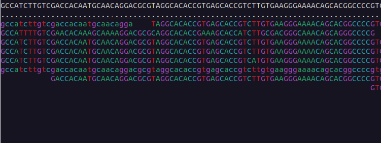
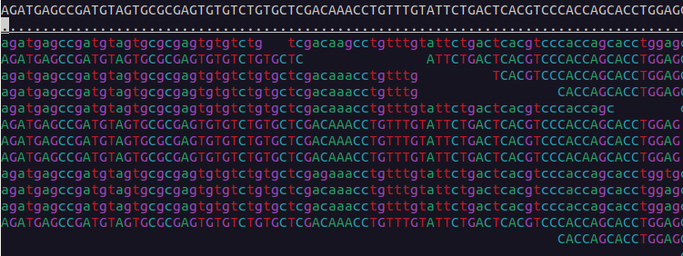
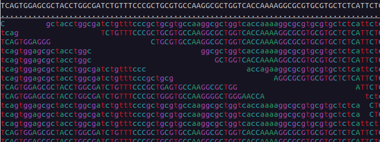
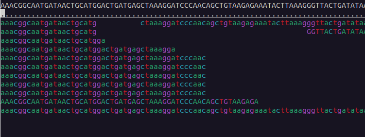
We can visualise the mapped data using samtools tview:
$ samtools tview bams/sample-1_bwa.bam reference/ninespine_rm.fa -p ctg7180000005484:13100You can find the instructions for its usage by typing the command name only (samtools tview) and pressing ? inside the program. Useful commands within the program are . and n. Find out what they mean.
Realignment around indels
One problem of bwa mem is that it aligns the reads separately and do not consider the alignment of other reads. This can cause errors around indels (=insertions and deletions). We use GATK to realign those regions although the developers of the tool say that this is no more necessary when using a pipeline like ours. I disagree with this and have seen the results with other GATK tools to change by realignment of the reads. Moreover, other tools use BAM files as such, and making the BAMs as good as possible is worthwhile.
Because of the decisions of the GATK development team, the realignment tools are no more a part of the GATK (v.4 and higher) packages. We use them from GATK v3. Due to licensing issues, CSC cannot provide these as a model and we have to use an installation of my own.
The process consists of two parts. First, we create a list of regions to realign:
$ gatk3=/projappl/project_2000598/bin/gatk3
$ ref=reference/ninespine_rm.fa
$ smp=sample-1
$ bams=bams

$ $gatk3 -T RealignerTargetCreator \
   -R ${ref} -I $bams/${smp}_bwa.bam -o $bams/${smp}.intervals
then, realign the BAM files around the target:
$ $gatk3 -T IndelRealigner \
   -R ${ref} -I $bams/${smp}_bwa.bam -targetIntervals $bams/${smp}.intervals -o $bams/${smp}_real.bam

$ samtools markdup $bams/${smp}_real.bam $bams/${smp}_mdup.bam
$ samtools index $bams/${smp}_mdup.bam
The last two commands mark the duplicates and index the resulting file.
Note that in the commands starting:
$ $gatk3 ...the first dollar sign is the prompt symbol and is not copied to your command, but the second dollar sign indicates that “$gatk3” is variable and must be copied to your command.
As a part of short-read sequencing, the samples undergo PCR amplification. As a result, the pool of fragments to be sequenced may contain PCR duplicates of exactly the same sequence. On the other hand, a cluster on the sequencing chip (where the reactions happen) may occasionally spread such that it forms two neighbouring spots containing the same sequence. These are called PCR and optical duplicates, respectively.
Such duplicates appear as independent reads in the data but, in reality, do not represent independent observations of the genome. The odds that two random fragments of a genome have exactly the same endpoints by chance (and then produce identical sequencing reads) are vanishingly small. Given that, the read-pairs with exactly the same end points are considered duplicates and all but one copy of them is marked as “duplicate”. The data are not removed but analysis methods aware of the practice do not consider them in calculations.
The information about duplicates is included in the FLAG field of SAM/BAM files. The format specification of SAM is at https://samtools.github.io/hts-specs/SAMv1.pdf, the FLAG field is explained on page 7.
Binary numbers are explained on EEB-021. In a FLAG, the zeros and ones can be seen as switches – ON vs OFF – such that the combination of switches makes the full binary number; for practical reasons, this binary number is converted to a decimal number for the samtools command. A useful tool to play with flags is at https://broadinstitute.github.io/picard/explain-flags.html. If we check “read is PCR or optical duplicate”, the SAM Flag is “1024”. We can read the instruction with the command:
$ samtools viewand learn that -f FLAG or --require-flags FLAG means “Only include in output reads that have all of the FLAGs present”. With that information, we can now select only those reads that have been marked as duplicates:
$ samtools view -f 1024 $bams/${smp}_mdup.bam | less -SThere are lots of them. We can select the first four of them and output four fields (look at the table above to see what these are):
$ samtools view -f 1024 $bams/${smp}_mdup.bam | head -4 | cut -f2,3,4,81187 ctg7180000005484 19207 19358
1123 ctg7180000005484 19294 19434
1107 ctg7180000005484 19358 19207
1171 ctg7180000005484 19434 19294First we notice that none of them has FLAG value “1024”. Pick the first of these, “1187”, and copy it to “SAM Flag” field on the “Decoding SAM flags” web page and click “Explain”. That should explain it. You can confirm all other flag values if still in doubt.
Next we notice that the numbers are repeated: “19358” is the last column on the 1st row, and the second last column on the 3rd row; the same for “19434” on the 2nd and 4th row.
These are mate pairs that we marked earlier and when marking reads as duplicates, mate pairs are always marked together.
We can confirm the duplicates visually:
$ samtools tview $bams/${smp}_mdup.bam $ref -p ctg7180000005484:19206
$ samtools tview $bams/${smp}_mdup.bam $ref -p ctg7180000005484:19357
The two reads with exactly the same start and end points are near the bottom.
Variant calling
In the variant calling, we approximately follow the GATK guidelines for “Germline short variant discovery (SNPs + Indels)”. GATK v.4+ is provided as a module on Puhti and we start with its tool HaplotypeCaller. You can see the tool documentation here.
Using the earlier approach, the command looks like this:
$ ref=reference/ninespine_rm.fa
$ smp=sample-1
$ bams=bams
$ gvcfs=gvcfs
$ mkdir $gvcfs

$ module load gatk

$ gatk HaplotypeCaller \
    -R ${ref} -I $bams/${smp}_mdup.bam \
    -O $gvcfs/${smp}.gvcf.gz -ERC GVCF
Here, the only optional parameter is -ERC GVCF that tells to the GVCF approach for reporting the confidence on non-variant sites. We’ll have a closer look on that elsewhere.
Note that two versions of GATK differ on the format for selecting the analysis tool: in GATK v.3 one has to use the parameter -T to select the tool (gatk3 -T <toolname>) but in GATK v.4 the tool name comes without any parameter (gatk4 <toolname>).
The run takes less than five minutes. You can look at the resulting file with less but a more formal way is to use the program bcftools from the “samtools” module:
$ less -S gvcfs/sample-1.gvcf.gz
$ bcftools view gvcfs/sample-1.gvcf.gz | less -S
you have to browse a few hundred rows down to see the calls. They start after “#CHROM …”.
Doing it all at once with SLURM
This seems like a lot of work to map and align a single sample and we may have hundreds of them in a study. Fortunately multiple commands can be collected into a script and this script may then be automated to handle multiple samples. Below is a naive approach to map all samples in the directory “fastq”. It works for our one sample but, with many more samples, the 15 minutes time limit of the partition “test” would quickly run out. Furthermore, the idea of computer cluster is to parallelise tasks (i.e. run them simultaneously), not to serialise the tasks as the loop over files below does.
Nevertheless, you can copy the script using the Heredoc format:
$ cat > map_and_call.sh << 'EOF'
#!/bin/bash
#SBATCH --time=15:00
#SBATCH --nodes=1
#SBATCH --ntasks=1
#SBATCH --cpus-per-task=2
#SBATCH --mem=6G
#SBATCH --partition=test
#SBATCH --account=project_2000598
#SBATCH --output=logs/map_and_call-%j.out

gatk3=/projappl/project_2000598/bin/gatk3
ref=reference/ninespine_rm.fa

fastq=fastq
bams=bams
gvcfs=gvcfs

module load bwa
module load gatk
module load samtools

ls $fastq/sample-*1.fq.gz | xargs -n1 -I% basename % _1.fq.gz | while read smp; do

  rgroup="@RG\tID:$smp\tLB:Lib\tSM:$smp\tPL:Plfm"

  bwa mem -t2 -R ${rgroup} ${ref} $fastq/${smp}_1.fq.gz $fastq/${smp}_2.fq.gz \
    | samtools fixmate -m - -  | samtools sort - -o $bams/${smp}_bwa.bam \
    && samtools index $bams/${smp}_bwa.bam

  $gatk3 -T RealignerTargetCreator \
    -R ${ref} -I $bams/${smp}_bwa.bam -o $bams/${smp}.intervals

  $gatk3 -T IndelRealigner \
    -R ${ref} -I $bams/${smp}_bwa.bam -targetIntervals $bams/${smp}.intervals -o $bams/${smp}_real.bam

  samtools markdup $bams/${smp}_real.bam $bams/${smp}_mdup.bam
  samtools index $bams/${smp}_mdup.bam

  gatk HaplotypeCaller \
    -R ${ref} -I $bams/${smp}_mdup.bam -O $gvcfs/${smp}.gvcf.gz -ERC GVCF

done

EOF
You can then create the log directory and check that the script looks good:
$ mkdir logs
$ less map_and_call.sh
If you are happy with that, you can submit it to the queue:
$ sbatch map_and_call.shand check how it progresses there:
$ squeue --meIf everything goes fine, in less than minutes the script should be ready and BAM and GVCF files are created in correct directories. You can browse the log file with the command:
$ less logs/map_and_call-*.outThe last part utilises the SLURM job scheduling system at Puhti. You can rehearse the vocabulary and concepts used at https://intscicom.biocenter.helsinki.fi/section5.html#running-jobs-on-a-linux-cluster
Short-read sequencing data are provided in FASTQ format that consists of a header line, a sequence line and a base-call quality line. The reads are aligned – or mapped – to a reference genome; the output of that is provided in SAM/BAM format that retains everything from the FASTQ and adds information about the mapping. In the variant calling, the differences between the sample and the reference are identified, reducing the size of the data dramatically. In the analysis of many samples, a common practice is to report the variants in GVCF format that 1) lists the observed differences in comparison to the reference genome and 2) reports the certainty that there are truly no variants in the intervening positions. The latter is important as seeing no variants can be caused by the true lack of variants in the existing data and lack of data to observe the variants.


