5. Inference of derived allele frequencies
After this practical, the students can infer ancestral alleles using an outgroup and use this information to infer derived allele frequencies directly from genotype data and using genotype likelihoods. They can explain why using genotype likelihoods is expected to be superior approach on low-coverage data.
Getting to Puhti
Get to your working directory:
$ WORK=/scratch/project_2000598
$ cd $WORK/$USER
If you are on a login node (if you access Puhti through a stand-alone terminal, you get to a login node; in the web interface, you can select either a login node or a compute node), start an interactive job (see sinteractive -h for the options):
$ # the command below is optional, see the text!
$ sinteractive -A project_2000598 -p small -c 2 -m 4000 -t 8:00:00We will utilise the SLURM job scheduling system at Puhti. You can rehearse the vocabulary and concepts used at https://intscicom.biocenter.helsinki.fi/section5.html#running-jobs-on-a-linux-cluster
Ancestral alleles in theory
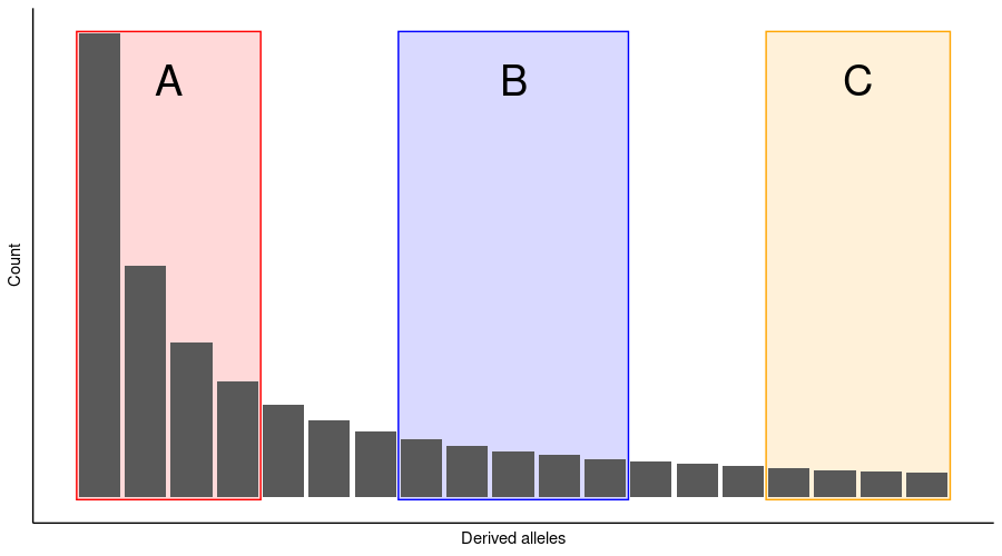
Many inferences of the coalescence process are based on the distributions of derived alleles. The derived allele means the new type generated by a mutation; the other allele type is called the ancestral allele.
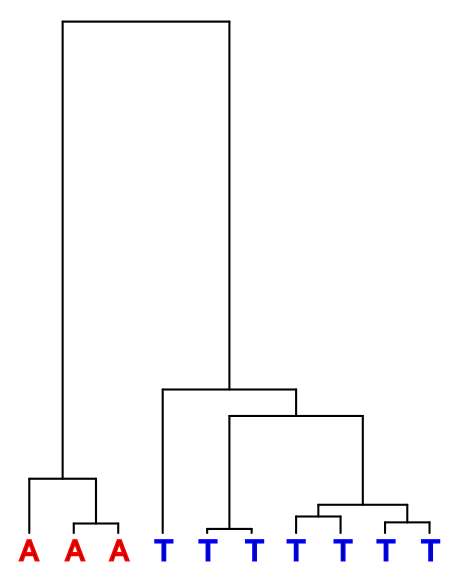
Suppose that we have observed three A’s and seven T’s at a specific genomic position among our ten samples. A hypothetical history for this site could be the following:
We assume parsimony and the simplest possible explanation, excluding the possibilities requiring multiple mutations. Then, to get this pattern, the mutation between A and T must have happened somewhere in the two top-most (longest) branches. How can we know whether A or T is the derived allele and whether we then have either three or seven derived alleles at this position?
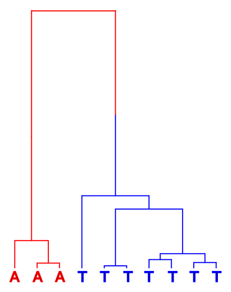
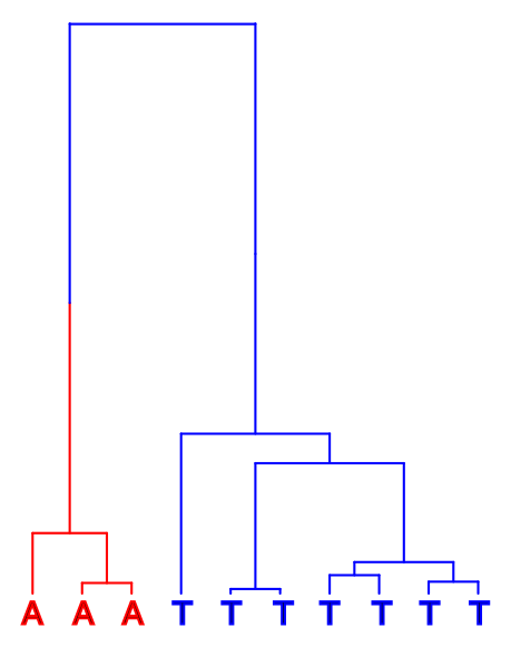
We cannot assume that the less common allele would be the derived one. The ancestral allele, or the top of the tree in the figures below, could either have been A (red) or T (blue):
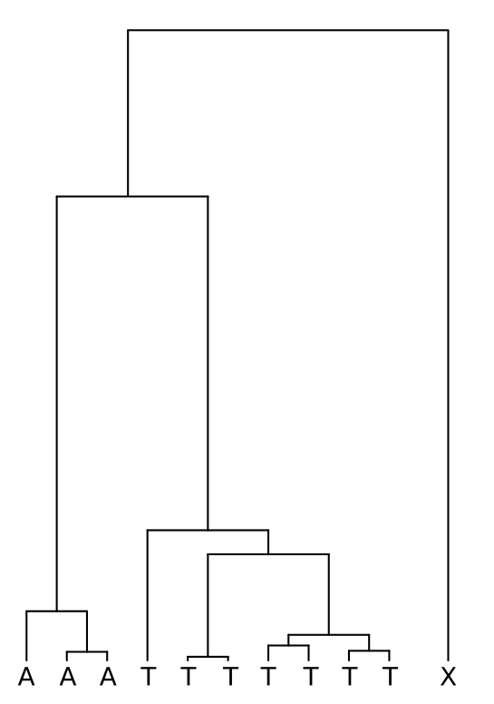
A simple approach to infer the ancestral allele is to use an outgroup that is with certainty outside of all the ingroup samples. In the figure below, this outgroup is marked with “X”: if X has allele A at this position, the most parsimonious solution is that the A was is the ancestral allele and it was mutated to T in one of the branches; conversely, if X has allele T, the ancestral allele is inferred to have been T. If X is something else but A or T (or if it’s an A/T heterozygote), the ancestral allele cannot be resolved.
There’s rarely a perfect outgroup and this approach is likely to produce some errors. First, the outgroup should be with certainty outside of the ingroup. That is difficult to guarantee and, for example, humans have genomic regions where orang-utans are our closest relative, not chimps or gorillas. On the other hand, the outgroup should not be too distant as then the possibilities of multiple independent mutations increase and the it would be possible, for example, that the true ancestral allele was T but it was independently mutated to A in the outgroup and in some of the ingroup samples; using the parsimony criterion, T would be incorrectly inferred as the derived allele.
Ancestral alleles in practice
As explained in the theory part, many analyses need to know which allele is ancestral and which is derived. This ordering of alleles is called “polarisation” and erroneously inferred allele states are “mis-polarised”. There are different ways to add the information about the ancestral allele (AA) into VCF files and we practice one of them below.
Our study data are from nine-spined sticklebacks, Pungitius pungitius. We use one sample of Sakhalin stickleback, Pungitius tymensis, to polarise our data. The use of sample only in the polarisation may introduce some errors e.g. due to incomplete lineage sorting (ILS) or multiple mutations on a site. However, P. tymensis should be of the right evolutionary distance to work nicely in the AA inference, i.e. not too close (increases ILS) and not too distant (increases multiple mutations).
This sample, PT-MOT-20, has been mapped and called previously. We copy the GVCF-file:
$ mkdir outgroup
$ cp $WORK/shared/outgroup/PT-MOT-20.gvcf.gz* outgroup/
and prepare the command to call it as VCF. I’m unaware of a perfect approach for calling the outgroup sample and the pipeline we use is a bit messy.
The first trick is to add parameters -L and --force-output-intervals in the GenotypeGVCFs command. This ensures that the positions for which we want to get the ancestral alleles (specified in the file 100_samples_rpm_snps.vcf.gz below) are called even if they are invariable in the sample in question. This gives us the command:
$ cat > genotype_outgroup_slurm.sh << EOF
#!/bin/bash
#SBATCH --time=15:00
#SBATCH --nodes=1
#SBATCH --ntasks=1
#SBATCH --cpus-per-task=1
#SBATCH --mem=5G
#SBATCH --partition=test
#SBATCH --account=project_2000598
#SBATCH --output=logs/genotype_outgroup-%j.out

module load gatk

gatk GenotypeGVCFs \
  -L vcfs/100_samples_rpm_snps.vcf.gz \
  --call-genotypes true \
  --force-output-intervals vcfs/100_samples_rpm_snps.vcf.gz \
  -R reference/ninespine_rm.fa \
  -V outgroup/PT-MOT-20.gvcf.gz \
  -O outgroup/PT-MOT-20.vcf.gz
EOF
Before we start the job, it may be necessary to index the file 100_samples_rpm_snps.vcf.gz again. bcftools index can write the index either in the CSI-format (default) or in the TBI-format (with the option -t). bcftools commands accept both index formats but the GATK tools only the latter. We can fix that with:
$ tabix vcfs/100_samples_rpm_snps.vcf.gz
 # OR
$ bcftools index -t vcfs/100_samples_rpm_snps.vcf.gz
After that, we can start the job with:
$ sbatch genotype_outgroup_slurm.shIt is useful to have a look on the output:
$ module load samtools
$ bcftools view -H outgroup/PT-MOT-20.vcf.gz | less -S
I would emphasise a few points visible here:
$ bcftools query -f '%CHROM\t%POS\t%REF\t%ALT\t%INFO/DP[\t%GT]\n' outgroup/PT-MOT-20.vcf.gz | headctg7180000005484 2377 G . 1 0/0
ctg7180000005484 3720 A . 2 0/0
ctg7180000005484 3722 A . . 0/0
ctg7180000005484 3731 A . . 0/0
ctg7180000005484 18700 G . 9 0/0
ctg7180000005484 18768 C . 3 0/0
ctg7180000005484 18874 C . 6 0/0
ctg7180000005484 18890 A C 8 1|1
ctg7180000005484 18917 C . 9 0/0
ctg7180000005484 18969 G . 15 0/0$ bcftools query -f '%CHROM\t%POS\t%REF\t%ALT\n' vcfs/100_samples_rpm_snps.vcf.gz | headctg7180000005484 2377 G A
ctg7180000005484 3720 A G
ctg7180000005484 3722 A G
ctg7180000005484 3731 A T
ctg7180000005484 18700 G T
ctg7180000005484 18768 C A
ctg7180000005484 18874 C T
ctg7180000005484 18890 A G
ctg7180000005484 18917 C A
ctg7180000005484 18969 G TFirst, the position 2377 is called in PT-MOT-20 but, as it doesn’t vary, no ALT allele is specified. We have that information 100_samples_rpm_snps.vcf.gz though. Second, the sequencing coverage (INFO/DP) is very low for the first sites in PT-MOT-20.vcf.gz. Can we trust the genotype based on one or two reads?
To resolve these issues, we do the following tricks. First, we filter the sites and include only those with enough sequencing coverage (-i 'INFO/DP>4'). Then, we output the fields CHROM, POS, REF and ALT for both files and additionally GT for PT-MOT-20. In addition to those, we create an “ID” for each site by merging the CHROM and POS fields: to make that ID to work correctly in sorting, the POS field is filled with leading zero:
$ bcftools query -i 'INFO/DP>4' -f '%CHROM\t%POS\t%REF\t%ALT[\t%GT]\n' outgroup/PT-MOT-20.vcf.gz \
   | awk '{OFS="\t";printf "%s.%09d\t",$1,$2; print $0}' > outgroup/PT-MOT-20.sites.tsv
The output looks like this
$ head outgroup/PT-MOT-20.sites.tsv ctg7180000005484.000018700 ctg7180000005484 18700 G . 0/0
ctg7180000005484.000018874 ctg7180000005484 18874 C . 0/0
ctg7180000005484.000018890 ctg7180000005484 18890 A C 1|1
ctg7180000005484.000018917 ctg7180000005484 18917 C . 0/0
ctg7180000005484.000018969 ctg7180000005484 18969 G . 0/0
ctg7180000005484.000019030 ctg7180000005484 19030 T . 0/0
ctg7180000005484.000019163 ctg7180000005484 19163 A . 0/0
ctg7180000005484.000019172 ctg7180000005484 19172 C . 0/0
ctg7180000005484.000019194 ctg7180000005484 19194 G . 0/0
ctg7180000005484.000019204 ctg7180000005484 19204 C . 0/0Bash commands typically use lexicographic order for sorting. Lexicographically, ‘1’ is before ‘5’ and thus ‘10’ is sorted before ‘5’; ‘0’ comes before ‘1’ and writing ‘05’ sorts ‘five’ before ‘ten’.
Above, printf command is used to add leading zeros to position numbers and then to merge the first two fields as an ID. This ensures that the IDs are correctly seen to be in order. You can test the behaviour of printf command with this:
$ echo ctg1 100 | awk '{printf "%s.%09d\n",$1,$2}'ctg1.000000100We’ll do a similar conversion for the second file
$ bcftools query -f '%CHROM\t%POS\t%REF\t%ALT\n' vcfs/100_samples_rpm_snps.vcf.gz \
   | awk '{OFS="\t";printf "%s.%09d\t",$1,$2; print $0}' > outgroup/100_samples.sites.tsv
and the output looks like this
$ head outgroup/100_samples.sites.tsv ctg7180000005484.000002377 ctg7180000005484 2377 G A
ctg7180000005484.000003720 ctg7180000005484 3720 A G
ctg7180000005484.000003722 ctg7180000005484 3722 A G
ctg7180000005484.000003731 ctg7180000005484 3731 A T
ctg7180000005484.000018700 ctg7180000005484 18700 G T
ctg7180000005484.000018768 ctg7180000005484 18768 C A
ctg7180000005484.000018874 ctg7180000005484 18874 C T
ctg7180000005484.000018890 ctg7180000005484 18890 A G
ctg7180000005484.000018917 ctg7180000005484 18917 C A
ctg7180000005484.000018969 ctg7180000005484 18969 G TWe can see that the first file doesn’t include all the sites present in the second file (the coverage was too low) but it doesn’t include any other sites either. The importance of the second file is that it contains also the ALT allele for all sites.
We can now match these two files based on the ID in the first column. The output of that looks like this:
$ join -j1 outgroup/100_samples.sites.tsv outgroup/PT-MOT-20.sites.tsv | head -5ctg7180000005484.000018700 ctg7180000005484 18700 G T ctg7180000005484 18700 G . 0/0
ctg7180000005484.000018874 ctg7180000005484 18874 C T ctg7180000005484 18874 C . 0/0
ctg7180000005484.000018890 ctg7180000005484 18890 A G ctg7180000005484 18890 A C 1|1
ctg7180000005484.000018917 ctg7180000005484 18917 C A ctg7180000005484 18917 C . 0/0
ctg7180000005484.000018969 ctg7180000005484 18969 G T ctg7180000005484 18969 G . 0/0We will feed this output to an awk command that processes the information one line at a time. The command looks like this:
$ join -j1 outgroup/100_samples.sites.tsv outgroup/PT-MOT-20.sites.tsv \
  | awk '$4==$8 && ($5==$9 || $9=="."){
    OFS="\t";
    if($10=="0/0" || $10=="0|0") {
      print $2,$3,$4,$5,$4
    } else if($10=="1/1" || $10=="1|1") {
      print $2,$3,$4,$5,$5
    } else {
      print $2,$3,$4,$5,"."
    }
   }' >  outgroup/AA.sites.tsv
In the first line of the awk command, we ensure that the REF alleles are the same ($4==$8) and the ALT alleles are either the same or missing in the second file (($5==$9 || $9==".")). In the following if-else commands, we do different actions depending on the genotype of PT-MOT-20 (that is $10). If that is “0/0”, the AA (ancestral allele) is the same REF ($4); if it is “1/1”, the AA is the same ALT ($5); otherwise, the AA is unknown (.).
We can see the output:
$ head -5 outgroup/AA.sites.tsv ctg7180000005484 18700 G T G
ctg7180000005484 18874 C T C
ctg7180000005484 18917 C A C
ctg7180000005484 18969 G T G
ctg7180000005484 19030 T A TYou can use the output of the join command and the awk command above to reason why the position 18890 is excluded.
This file now contains the fields CHROM, POS, REF, ALT and INFO/AA. The first four are already in our data file and are just used to ensure that the fifth field, INFO/AA, is added to exactly right place in the data.
We compress and index the file:
$ bgzip outgroup/AA.sites.tsv
$ tabix -s1 -b2 -e2 outgroup/AA.sites.tsv.gz
We need to define what our new “INFO/AA” field means and we write the description in a file:
$ echo '##INFO=<ID=AA,Number=1,Type=Character,Description="Ancestral allele">' > outgroup/hdr.txtGiven that, we can now annotate our existing VCF file with the new information. The command specifies the source of annotation information (-a), its format (-c) and the description to be added to the header (-h). We add this annotation to 100_samples_rpm_snps.vcf.gz and call the output file 100_samples_rpm_snps_AA.vcf.gz:
$ bcftools annotate -a outgroup/AA.sites.tsv.gz -c CHROM,POS,REF,ALT,INFO/AA -h outgroup/hdr.txt \
  -Oz -o vcfs/100_samples_rpm_snps_AA.vcf.gz vcfs/100_samples_rpm_snps.vcf.gz
$ bcftools index vcfs/100_samples_rpm_snps_AA.vcf.gz
We can check that the AA field is indeed described in the header (the order doesn’t matter and it’s towards the bottom of the header):
$ bcftools view -h vcfs/100_samples_rpm_snps_AA.vcf.gz | less -Sand given in the INFO section (it’s the last item):
$ bcftools view -H -r ctg7180000005484:18700 vcfs/100_samples_rpm_snps_AA.vcf.gz | lessWe can now use the “INFO/AA” field for filtering and count on how many positions the AA is identical to REF and ALT, how many positions lack AA:
$ bcftools view -H -i 'INFO/AA=REF' vcfs/100_samples_rpm_snps_AA.vcf.gz | wc -l
$ bcftools view -H -i 'INFO/AA=ALT' vcfs/100_samples_rpm_snps_AA.vcf.gz | wc -l
$ bcftools view -H -i 'INFO/AA="."' vcfs/100_samples_rpm_snps_AA.vcf.gz | wc -l
$ bcftools view -H vcfs/100_samples_rpm_snps_AA.vcf.gz | wc -lDerived alleles
Given the ancestral alleles, the derived allele frequencies (DAF) can be computed with vcftools. For comparison, we also compute them with angsd that works differently and computes the statistics directly from BAM files.
First, we create a list of sample names (for vcftools) and BAM files (for angsd) for two populations:
$ mkdir sfs

$ for pop in FIN-RYT RUS-MAS; do
    grep $pop plink/sample_names.txt | cut -c9- > sfs/${pop}.txt
    cat sfs/${pop}.txt  | xargs -n1 -I% ls $WORK/shared/bams/%_mdup.bam > sfs/${pop}.bams
done
We then use vcftools to compute allele counts (--counts2) per variable position for the subset of samples (--keep); it is important to specify --derived such that the counts are correctly polarised:
$ module load vcftools

$ for pop in FIN-RYT RUS-MAS; do
    vcftools --gzvcf vcfs/100_samples_rpm_snps_AA.vcf.gz --keep sfs/${pop}.txt --counts2 --derived --out sfs/${pop}_vcftools
done
One can see the output of vcftools:
$ less sfs/FIN-RYT_vcftools.frq.count The column names are specified in the header line. All our variants are binary (N_ALLELES==2) but the number of samples with data varies and N_CHR is not always 20. The last two columns are the counts for two alleles.
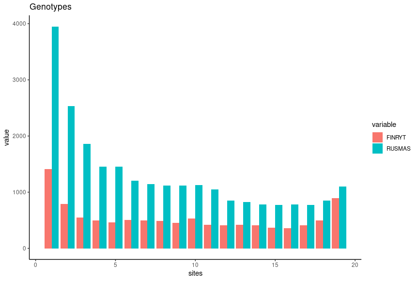
We can plot the SFS for the two populations with R. Below, we only keep the sites with data for all samples (N_CHR) and then count the number of derived alleles (N_DA). In the barplot, the first (N_DA==0) and the last (N_DA==20) column are omitted and only the segregating sites are considered:
setwd(paste0("/scratch/project_2000598/",Sys.getenv("USER")))

library(ggplot2)
library(reshape2)
library(dplyr)
library(cowplot)

cnames <- c("CHROM","POS","N_ALL","N_CHR","N_AA","N_DA")

ryt.vcftools <- read.table("sfs/FIN-RYT_vcftools.frq.count",skip=1,col.names = cnames)
mas.vcftools <- read.table("sfs/RUS-MAS_vcftools.frq.count",skip=1,col.names = cnames)

ryt.gt <- ryt.vcftools %>% filter(N_CHR==20)  %>% count(N_DA) %>% select(n) %>% t()
mas.gt <- mas.vcftools %>% filter(N_CHR==20)  %>% count(N_DA) %>% select(n) %>% t()

gt <- data.frame(sites=1:19,FINRYT=ryt.gt[2:20],RUSMAS=mas.gt[2:20])
gt.df <- melt(gt,id.vars = "sites")

pl1 <- ggplot(gt.df) +
    geom_col(aes(x = sites,y=value,fill=variable),position = "dodge")+
    theme_classic()+
    ggtitle("Genotypes")

pl1The output resembles the expectation based on the theory, especially for the population RUS-MAS.
Genotype likelihoods
We will then do the same using ANGSD.
ANGSD is specifically designed for low-coverage data where the genotypes may be incorrectly inferred due to the small number of observations. When using the inferred genotypes, counting happens on integers: the genotypes “0/0”, “0/1” and “1/1” have exactly 0, 1 and 2 ALT alleles. ANGSD doesn’t do that but considers the possibility that a site doesn’t show any derived allele (and its inferred genotype is “0/0”) because of low sequencing coverage. To correct for the error, ANGSD sets a small likelihood also for the genotype “0/1”. As a results, ANGSD doesn’t use genotypes (GT) but genotype likelihoods (GL).
We first reconstruct an ancestral genome using the BAM data for PT-MOT-20:
$ module load angsd

$ bam=$WORK/shared/outgroup/PT-MOT-20_mdup.bam
$ out=reference/PT-MOT-20

$ angsd -doFasta 2 -explode 1 -doCounts 1 -minQ -1 -i $bam -out $out
$ samtools faidx $out.fa.gz
If you look at the resulting FASTA file:
$ less reference/PT-MOT-20.fa.gzyou can see that there’s lots of missing information due to poor sequencing coverage. It gets better further down though.
You can compare the FASTA index files:
$ head reference/PT-MOT-20.fa.gz.fai
$ head reference/ninespine_rm.fa.fai
and learn that the contigs in the two files are equally long. The ancestral genome thus provides the inferred ancestral state for every site in the reference genome (with the exception of sites with missing data).
To make the two analyses comparable, we utilise the positive mask also with ANGSD. The program requires a sligthly different format and has an own indexing approach. The second file simply lists the contigs we want include:
$ zcat reference/ninespine_posmask.bed.gz | awk '{OFS="\t";print $1,$2+1,$3}' > reference/ninespine_posmask.tab
$ angsd sites index reference/ninespine_posmask.tab
$ cut -f1 reference/ninespine_posmask.tab | uniq > reference/ninespine_posmask_ctgs.txt
With those, we can run angsd for the two populations. The likelihoods needed for SFS analyses are computed with the ANGSD option -doSaf 1:
$ ref=reference/ninespine_rm.fa
$ anc=reference/PT-MOT-20.fa.gz

$ for pop in FIN-RYT RUS-MAS; do
    angsd -gl 2 -doSaf 1 -b sfs/${pop}.bams -ref $ref -anc $anc -out sfs/$pop -uniqueOnly 1 -minMapQ 1 -minQ 20 -minInd 10 -sites reference/ninespine_posmask.tab -rf reference/ninespine_posmask_ctgs.txt
done
Look for the description of the command parameters at the ANGSD website.
This only computes the genotype likelihoods and we need to run realSFS to estimate the site frequencies:
$ for pop in FIN-RYT RUS-MAS; do
    realSFS sfs/${pop}.saf.idx > sfs/${pop}_angsd.sfs
done
One can see the output of realSFS:
$ less sfs/FIN-RYT_angsd.sfs This is simply a list of 21 numbers, the numbers telling how many times 0, 1, 2, …, 20 copies of a derived allele is observed at the variant positions.
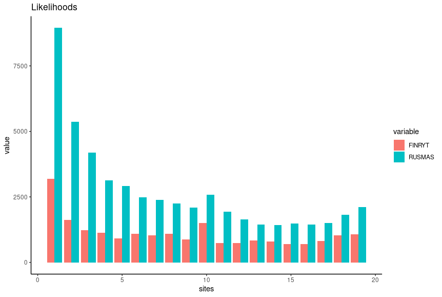
We can plot the SFS for the two populations with R. Again, the first (zero copies) and the last (20 copies) value are omitted and only the segregating sites are considered:
ryt.angsd <- read.table("sfs/FIN-RYT_angsd.sfs")
mas.angsd <- read.table("sfs/RUS-MAS_angsd.sfs")

ryt.gl <- t(ryt.angsd)[,1]
mas.gl <- t(mas.angsd)[,1]

gl <- data.frame(sites=1:19,FINRYT=ryt.gl[2:20],RUSMAS=mas.gl[2:20])
gl.df <- melt(gl,id.vars = "sites")

pl2 <- ggplot(gl.df) +
    geom_col(aes(x = sites,y=value,fill=variable),position = "dodge")+
    theme_classic()+
    ggtitle("Likelihoods")

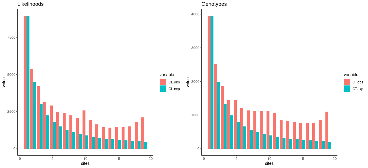
pl2 The output looks similar to one produced with vcftools but the numbers are generally higher.
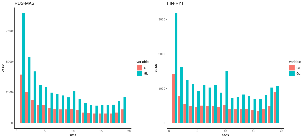
We can see that by comparing the GT and GL estimates for the same populations:
mas <- data.frame(sites=1:19,GT=mas.gt[2:20],GL=mas.gl[2:20])
mas.df <- melt(mas,id.vars = "sites")

pl3 <- ggplot(mas.df) +
    geom_col(aes(x = sites,y=value,fill=variable),position = "dodge")+
    theme_classic()+
    ggtitle("RUS-MAS")

ryt <- data.frame(sites=1:19,GT=ryt.gt[2:20],GL=ryt.gl[2:20])
ryt.df <- melt(ryt,id.vars = "sites")

pl4 <- ggplot(ryt.df) +
    geom_col(aes(x = sites,y=value,fill=variable),position = "dodge")+
    theme_classic()+
    ggtitle("FIN-RYT")

plot_grid(pl3,pl4,ncol=2)When comparing GL and GT-bases estimates, we can see that the difference is the greatest for singletons that are the most difficult category to estimate using the GT data.
A worrying sign is the peak at AF=0.5, i.e. at the number of sites having 10 copies of the derived allele. This pattern is often created by errors in the data and e.g. all samples being heterozygous because of segmental duplications and reads mapping to wrong places. Typically we would also expect the counts to decrease towards the right. In some circumstances, there can be natural reasons for the last counts to increase slightly, but the pattern is more often generated by wrong polarised SNPs and some counts moving from the extreme left to the extreme right.
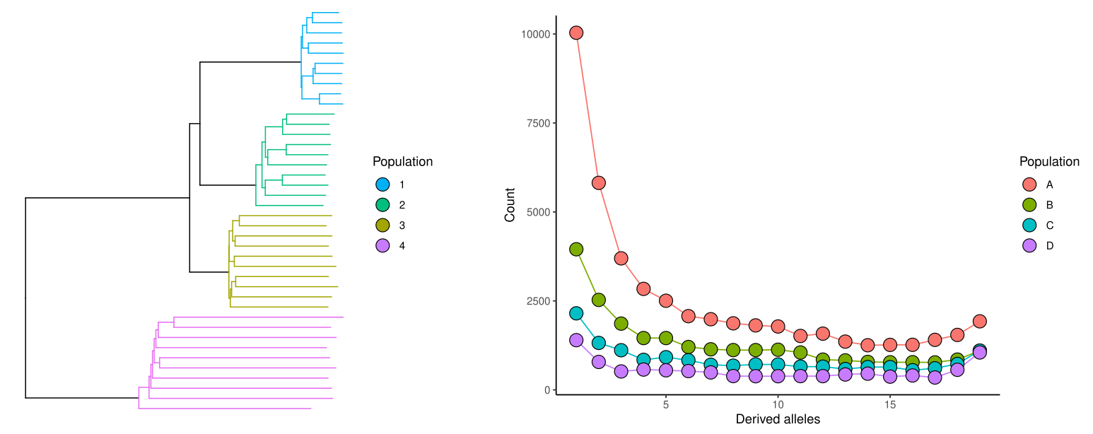
If we consider the number of singletons correct and then draw the expected values for all other categories based on that (rehearse the theory if you don’t remember how this is done), we can see the observed and expected distributions don’t match too well:
They don’t need to match perfectly if the population hasn’t evolved under the perfect WFM – which is highly likely true.
Although these examples may look discouraging, generally ANGSD is considered a superior approach in cases with fairly modest sequencing coverage and is widely used to compute SFS for demographic analyses.
Genotype likelihoods explained
We can have a glimpse on how ANGSD works by looking at our example data. We can plot the beginning of the GT data:
$ vcftools --gzvcf vcfs/100_samples_rpm_snps_AA.vcf.gz --keep sfs/RUS-MAS.txt --counts2 --derived -c | headCHROM POS N_ALLELES N_CHR {COUNT}
ctg7180000005484 18700 2 10 8 2
ctg7180000005484 18874 2 18 13 5
ctg7180000005484 18917 2 18 11 7
ctg7180000005484 18969 2 20 20 0
ctg7180000005484 19030 2 20 12 8
ctg7180000005484 19163 2 20 12 8
ctg7180000005484 19172 2 20 12 8
ctg7180000005484 19194 2 20 14 6
ctg7180000005484 19204 2 20 20 0and see that the position 19030 is the first one that has data for all samples (N_CHR==20) and alleles segregate (last two columns are not 20 and 0). We can extract that position from the GL data and convert the log10 values to decimal numbers:
$ realSFS print sfs/RUS-MAS.saf.idx -r ctg7180000005484:19030 2> /dev/null | awk '{for(i=3;i<24;i+=1){print i-3,10^$i}}'0 0
1 0
2 0
3 0
4 0
5 0
6 2.12337e-20
7 0.025131
8 1
9 0.000495936
10 1.53847e-08
11 1.07732e-14
12 0
13 0
14 0
15 0
16 0
17 0
18 0
19 0
20 0The output prints the copy number of the derived allele and the likelihood for this site having that many copies. We can see that the eighth copy has the value “1” and is chosen as the most likely copy number (as was in the GT data) but also the neighbouring count numbers get a small likelihood. With that, ANGSD can take into account teh uncertainty in the data and correct for the genotype-calling errors caused by the low sequencing depth.
Theta statistics
In addition to SFS estimation, genotype likelihoods make a big difference in analyses of theta statistics (i.e nucleotide diversity) and many selection statistics. The likelihoods for those analyses are computed with realSFS saf2theta. The analysis requires the SFS estimate that we computed above as a prior (option -sfs). The command is then:
$ for pop in FIN-RYT RUS-MAS; do
    realSFS saf2theta sfs/${pop}.saf.idx -sfs sfs/${pop}_angsd.sfs  -outname sfs/$pop
done
Given the new likelihood files, the theta estimates are computed as:
$ for pop in FIN-RYT RUS-MAS; do
    thetaStat do_stat sfs/${pop}.thetas.idx
done
We can look at the output:
$ column -t sfs/RUS-MAS.thetas.idx.pestPG | less -SThe ANGSD documentation says about this the following:
The .pestPG file is a 14 column file (tab seperated). The first column contains information about the region. The second and third column is the reference name and the center of the window.
We then have 5 different estimators of theta, these are: Watterson, pairwise, FuLi, fayH, L. And we have 5 different neutrality test statistics: Tajima’s D, Fu&Li F’s, Fu&Li’s D, Fay’s H, Zeng’s E. The final column is the effetive number of sites with data in the window.
If we are interested in \(\pi\), also known as Tajima’s \(\theta\) estimator, we have to consider the fifth column. The file contains the number of pairwise differences between sequences without correcting for the number of sites in the sequence. We can convert these counts as “differences per site” by dividing them by the sequence length (given after removing some sites due to positive mask filtering or ANGSD’s internal filtering) in the last (14th) column:
$ tail -n+2 sfs/RUS-MAS.thetas.idx.pestPG | awk '{t+=$5;s+=$14}END{print t/s}'
$ tail -n+2 sfs/FIN-RYT.thetas.idx.pestPG | awk '{t+=$5;s+=$14}END{print t/s}'
For comparison, we can do the same using the inferred genotypes with vcftools. To correctly take into account the impact of previous site filtering, we should do that using the option --site-pi. For that, we need to know the true length of our reference genome after the filtering and can do it by summing the lengths of the positively masked regions:
$ zcat reference/ninespine_posmask.bed.gz | awk '{s+=$3-$2}END{print s}'8670242The output of vcftools --site-pi, that is the estimate of \(\pi\) for all the variant positions, looks like this
$ vcftools --gzvcf vcfs/100_samples_rpm_snps_AA.vcf.gz --keep sfs/RUS-MAS.txt --site-pi -c | headCHROM POS PI
ctg7180000005484 2377 -nan
ctg7180000005484 3720 -nan
ctg7180000005484 3722 -nan
ctg7180000005484 3731 -nan
ctg7180000005484 18700 0.355556
ctg7180000005484 18768 0
ctg7180000005484 18874 0.424837
ctg7180000005484 18890 0.424837
ctg7180000005484 18917 0.503268We can see that the estimates include “nan” values for the sites with all missing data and those have to excluded from the final counts.
We could write the output to a file but can here do the computation on the fly:
$ vcftools --gzvcf vcfs/100_samples_rpm_snps_AA.vcf.gz --keep sfs/RUS-MAS.txt --site-pi -c | grep -v nan | awk '{s+=$3}END{print s/8670242}'Note that vcftools reports the estimates for all variant sites but doesn’t know the length of the sequence. Above, we sum the counts and divide the sum by the length that we computed above.
We can see that the \(\pi\) estimates using the GT and GL data differ. However, the estimates for the two populations are in the line and the relative differences between the populations is fairly similar.
2D SFS
We have so far looked at SFSs for single populations. They can be computed for multiple populations and those for two populations are commonly used in demographic analyses with dadi and the related method moments.
A 2D SFS for our two populations can be inferred with the command:
$ realSFS sfs/FIN-RYT.saf.idx sfs/RUS-MAS.saf.idx > sfs/FIN-RYT.RUS-MAS.sfsExamples of typical 2D SFSs can be seen in the moments website and in figures below.
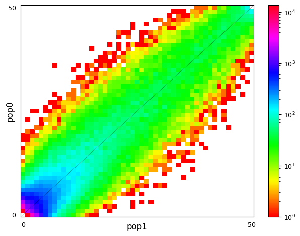
The concept is quite intuitive. Let’s assume that we have large population and then divide this into two smaller populations, 1 and 2. If we immediately study the allele frequencies in the two populations and observe e.g. AF=0.2 in population 1, we can expect the same locus a similar allele frequency in population 2: the count for that locus in the figure would then have the x coordinate 0.2 and the y coordinate close to 0.2 and fall somewhere close to the diagonal of te 2D plot. The same happens at other loci and the AFs in pop1 and pop2 correlate strongly, making the diagonal as in the left plot.
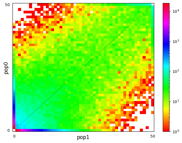
After some divergence, the AFs in population 1 and 2 start differ due to genetic drift and points in the 2D plot move further away from the diagonal. That can be seen in the right plot. In dadi and moments analyses, one tries to find demographic parameters for the divergence of the two populations that produce a 2D SFS looking similar to the observed one.
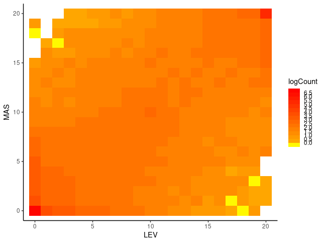
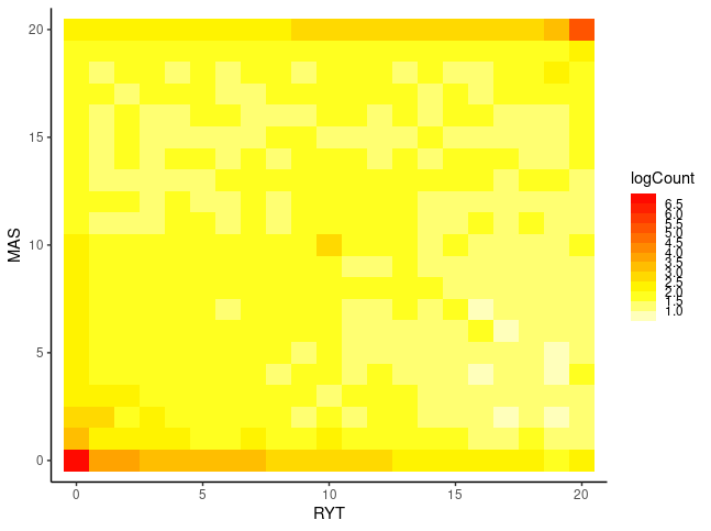
Our data are very small for this purpose and, moreover, FIN-RYT and RUS-MAS are so highly diverged that the 2D SFS contains little information. I replicated the ANGSD SFS inference for RUS-LEV, a population more closely related with RUS-MAS, and plotted the heatmap plots with R:
sfs=read.table("sfs/FIN-RYT.RUS-MAS.sfs")
data=expand.grid(X=0:20,Y=0:20)
data$logCount=log10(t(sfs))

ggplot(data) +
  geom_tile(aes(X,Y,fill=logCount))+
  scale_fill_stepsn(colours = rev(heat.colors(15)), breaks = seq(0,7,0.5) ,na.value = "white")+
  theme_classic() + coord_cartesian(xlim=c(0,20),ylim=c(0,20)) +
  xlab("RYT")+ylab("MAS")

sfs=read.table("sfs/RUS-LEV.RUS-MAS.sfs")
data=expand.grid(X=0:20,Y=0:20)
data$logCount=log10(t(sfs))

ggplot(data) +
  geom_tile(aes(X,Y,fill=logCount))+
  scale_fill_stepsn(colours = rev(heat.colors(15)), breaks = seq(0,7,0.5) ,na.value = "white")+
  theme_classic() + coord_cartesian(xlim=c(0,20),ylim=c(0,20)) +
xlab("LEV")+ylab("MAS")One of the files is missing. If you want to run the R cose, you have to generate the second SFS with the command:
$ realSFS sfs/RUS-LEV.saf.idx sfs/RUS-MAS.saf.idx > sfs/RUS-LEV.RUS-MAS.sfs Despite the limitations of the data and a very different colour scale, the plots have some resemblence to the exmaples from the moments website. In the left plot, a significant proportion of the sites segregate and the information is in the middle of the plot. In the right plot, a large fraction of the sites are in the outer-most columns and rows, meaning that the site is fixed in one population (AF=0 or AF=20) and segregates in the other or is also fixed (corners).
ANGSD is probably the best method for ingferring 2D SFSs for dadi and moments analyses.
Many population genetic analysis methods are based on the frequncies of derived alleles among the samples. Although the derived allele is by definition younger than the ancestral allele, it is not necesaarily the less frequent one. The derived alleles can be indetified by resolving the ancestral alleles.
Genotypes inferred from low-coverage data – widely used in population genetics – contain errors. ANGSD is a method specifically designed for low-coverage data and takes into account the uncertainty of the data by not only considering the best genotype but the likelihoods of multiple alternative genotypes. The downside of the approach is that the anlyses are slower and the intermediate files are much larger.
