8. Demographic inference with MSMC (and conservations genetics)

Learning outcome

After this chapter, the students can reproduce basic inference of demographic history using MSMC2 and MSMC-IM and visualise the results with R. They can also describe the effect of central parameters and draw conclusions from alternative \(N_e\), \(m\) and \(M\) trajectories.

Getting to Puhti

Get to your working directory:

$ WORK=/scratch/project_2000598
$ cd $WORK/$USER

If you are on a login node (if you access Puhti through a stand-alone terminal, you get to a login node; in the web interface, you can select either a login node or a compute node), start an interactive job (see sinteractive -h for the options):

$ # the command below is optional, see the text!
$ sinteractive -A project_2000598 -p small -c 2 -m 4000 -t 8:00:00

These practicals contain relatively heavy computation the work should be done on a compute node or using SLURM jobs.

Demographic inference wit MSMC2

We estimate the demographic history, i.e. the historical effective population size, with MSMC2. MSMC2 has a very specific data format and provides helper applications to convert the more traditional data to its own format.

Data conversion

Make a new directory for the analyses and link the shared directories containing the BAM files and the reference sequence for LG3:

$ cd $WORK/$USER

$ mkdir -p msmc/vcfs msmc/masks
$ cd msmc

$ ln -s $WORK/shared/msmc/bams .
$ ln -s $WORK/shared/msmc/ref .
$ ls -lh bams/
$ ls -lh ref/

Note that ref/ directory also contains a BED file defining the positive mask for LG3.

For the conversion, create a SLURM script that calls the variant positions from a BAM file and simultaneously creates a mask file that indicates which regions of the genome were callable. The script uses bamCaller.py from the msmc-tools package:

$ cat > call_bam.sh << 'EOF'
#!/bin/bash
#SBATCH --time=15:00
#SBATCH --nodes=1
#SBATCH --ntasks=1
#SBATCH --cpus-per-task=1
#SBATCH --mem=2G
#SBATCH --partition=test
#SBATCH --account=project_2000598
#SBATCH --output=../logs/call_bam-%j.out

module load python-data
module load samtools 

bamcaller=/projappl/project_2000598/sw/msmc-tools/bamCaller.py

smp=$1

chrom=LG3
dpt=$(samtools depth -r LG3 bams/${smp}_LG3.bam | awk '{sum += $3} END {print sum / NR}')

bcftools mpileup -q 20 -Q 20 -C 50 -Ou -r ${chrom} -f ref/NSPV7.fa.gz bams/${smp}_LG3.bam \
 | bcftools call -c -V indels | $bamcaller $dpt masks/${smp}.${chrom}.mask.bed.gz \
 | bgzip -c > vcfs/${smp}.${chrom}.vcf.gz

EOF

and then start the job:

$ sbatch call_bam.sh FIN-KAR-33

Once completed (it takes a few minutes), the resulting VCF looks pretty normal:

$ module load samtools 
$ bcftools query -f '%CHROM\t%POS\t%REF\t%ALT[\t%GT]\n' vcfs/FIN-KAR-33.LG3.vcf.gz | head

This VCF alone does not provide enough information for the analysis: MSMC2 is a Hidden Markov Model which uses the density of heterozygous sites (1/0 genotypes) to estimate the time to the most recent common ancestor. For a density you need not only a numerator but also a denominator, which in this case is the number of non-heterozygous sites, typically homozygous reference alleles. Homozygous reference alleles are naturally not shown in a VCF file. More seriously, we do not know which regions had not enough coverage or had too low quality for the genotypes to be called.

This information is contained in the mask-files, computed for each sample. The first lines of such a mask look like this:

$ less masks/FIN-KAR-33.LG3.mask.bed.gz | head

You can now either run the same script for all the other BAM files (in total ten) or copy the files as shown below. If you run the calculations by yourself, note that the “test” queue doesn’t allow more than one running and one waiting job. You could modify the script and send the jobs to the “small” queue; depending on the demand, they could all run very quickly or sit waiting in the queue.

These commands copy the precomputed data:

$ cp $WORK/shared/msmc/vcfs/* vcfs/
$ cp $WORK/shared/msmc/masks/* masks/

As we now have the mask files and VCF files for each sample, we can combine these into one file. This should be done separately for each chromosome and here we do it just for LG3. In the process, we also include the positive mask that has been precomputed as explained earlier in the course:

$ module load python-data
$ module load samtools 

$ mkdir multi
$ genmulti=/projappl/project_2000598/sw/msmc-tools/generate_multihetsep.py

$ $genmulti \
--mask=masks/FIN-KAR-33.LG3.mask.bed.gz \
--mask=masks/FIN-KAR-34.LG3.mask.bed.gz \
--mask=masks/FIN-RYT-PP43.LG3.mask.bed.gz \
--mask=masks/FIN-RYT-PP50.LG3.mask.bed.gz \
--mask=masks/RUS-KRU-25.LG3.mask.bed.gz \
--mask=masks/RUS-KRU-5.LG3.mask.bed.gz \
--mask=masks/RUS-LEV-B13.LG3.mask.bed.gz \
--mask=masks/RUS-LEV-F4M.LG3.mask.bed.gz \
--mask=masks/RUS-MAS-48.LG3.mask.bed.gz \
--mask=masks/RUS-MAS-5.LG3.mask.bed.gz \
--mask=ref/LG3_posmask.bed.gz \
vcfs/FIN-KAR-33.LG3.vcf.gz vcfs/FIN-KAR-34.LG3.vcf.gz \
vcfs/FIN-RYT-PP43.LG3.vcf.gz vcfs/FIN-RYT-PP50.LG3.vcf.gz \
vcfs/RUS-KRU-25.LG3.vcf.gz vcfs/RUS-KRU-5.LG3.vcf.gz \
vcfs/RUS-LEV-B13.LG3.vcf.gz vcfs/RUS-LEV-F4M.LG3.vcf.gz \
vcfs/RUS-MAS-48.LG3.vcf.gz vcfs/RUS-MAS-5.LG3.vcf.gz > multi/LG3.multihetsep.txt

The first lines of the resulting “multihetsep” file should look like this:

$ less -S multi/LG3.multihetsep.txt

This is the input file for MSMC2. The first two columns denote chromosome and position of a segregating site within the samples. The fourth column contains the 20 alleles in the 10 samples in our analysis. When there are multiple patterns separated by a comma, it means that phasing information is ambiguous, so there are multiple possible phasings. As our data are not phased, this happens a lot.

The third column contains the number of informative (called) sites since the previous segregating site, including the current site. So for example, in the first row above, the first segregating site is at position 61041, but not all 61,041 sites up to that site were called homozygous reference, but only 113. This is very important for MSMC2, because it would otherwise assume that there was a huge homozygous segment spanning from 1 through 61,041.

Important

Computer programs typically have “dependencies” and utilise functions provided by “libraries” or “packages” written by others. An example of those are the R libraries loaded in the beginning of the R scripts. The programs provided as modules on Puhti should come with all the necessary dependencies and no extra libraries need to be loaded. However, some programs used on the course are not provided as loadable modules and have been installed manually in a specific directory. generate_multihetsep.py above is one of them.

Many Python program utilise functions provided by NumPy and SciPy packages. Although they are widely used, they are not provided by default and have to loaded separately by the Python programs. generate_multihetsep.py does that and then utilises numerical routines provided by the two packages. On Puhti, these NumPy and SciPy (and other similar packages) are not available by default but can be loaded with the module python-data.

$ module load python-data

Demographic history with MSMC2

MSMC2’s purpose is to estimate coalescence rates between haplotypes through time. This can then be interpreted for example as the inverse effective population size through time. If the coalescence rate is estimated between subpopulations, another interpretation would be how separated the two populations became through time. Below, we will use both interpretations.

We had two samples per population, each having two chromosomes, in the order FIN-KAR, FIN-RYT, RUS-KRU, RUS-LEV and RUS-MAS. When running msmc2, one needs to specify which chromosomes are included in the analysis, starting the count from zero. The two FIN-KAR samples are the chromosomes 0-3. With that, we can run msmc2 for the population FIN-KAR as:

$ module load msmc2
$ mkdir output

$ msmc2 -p 1*2+25*1+1*2+1*3 -I 0,1,2,3 -o output/FINKAR_LG3 multi/LG3.multihetsep.txt &> output/FINKAR_LG3.runlog

Of the command options, -p defines the time segment patterning and could it be omitted here as the given pattern is identical to the program’s default value. The pattern defines 32 time segments, grouped as 1*2+25*1+1*2+1*3, which means that the first 2 segments are joined (forcing the coalescence rate to be the same in both segments), then 25 segments each with their own rate, and then again two groups of 2 and 3, respectively. The run time and memory usage of MSMC2 scale quadratically with the number of time segments.

In the analyses of small amounts of data, one should possibly reduce the number of segments to avoid overfitting. With our data, the smaller number of segments caused issues and we use the default option.

The -o option denotes an output prefix. The three files generated by MSMC2 will be called like this prefix with endings .final.txt, .loop.txt and .log.

The -I option denotes the 0-based indices of the haplotypes analysed. In our case we have 4 haplotypes from the two FIN-KAR individual, The last argument to MSMC2 is the multihetsep file. Normally one should run the analysis on all chromosomes, and in that case one would simply give all the files in a row or use wildcard characters.

There are additional parameters as explained in the program documentation.

Once that is computed, we can view the contents of the file:

$ column -t output/FINKAR_LG3.final.txt | less -S

This may look cryptic but is consistent with the idea of segmenting the time and then estimating the coalescence rate within each segment. The first column denotes a simple index of all time segments, the second and third indicate the scaled start and end time for each time interval. The last column contains the scaled coalescence rate estimate in that interval.

This needs to be replicated for the other populations and the pair indices (-I) need to be modified for each command:

$ msmc2 -I 4,5,6,7 -o output/FINRYT_LG3 multi/LG3.multihetsep.txt &> output/FINRYT_LG3.runlog 

$ msmc2 -I 8,9,10,11 -o output/RUSKRU_LG3 multi/LG3.multihetsep.txt &> output/RUSKRU_LG3.runlog 

$ msmc2 -I 12,13,14,15 -o output/RUSLEV_LG3 multi/LG3.multihetsep.txt &> output/RUSLEV_LG3.runlog 

$ msmc2 -I 16,17,18,19 -o output/RUSMAS_LG3 multi/LG3.multihetsep.txt &> output/RUSMAS_LG3.runlog 

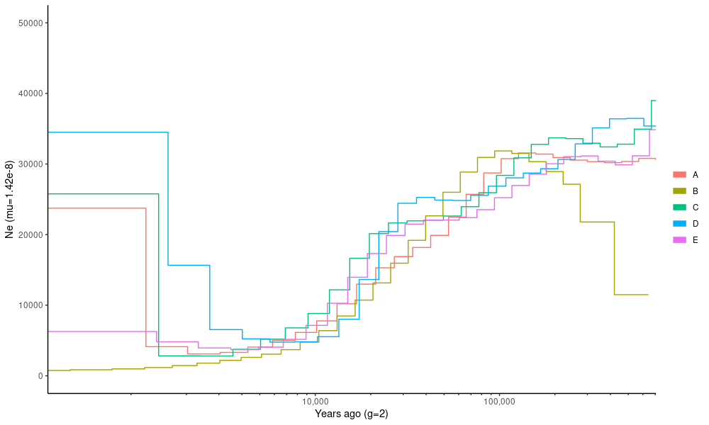
Once these all are computed, we can plot them. Below, we assume a generation time (gt) of two years and mutation rate (mu) of \(1.42\times 10^{-8}\) substitutions per site per generation:

setwd(paste0("/scratch/project_2000598/",Sys.getenv("USER"),"/msmc"))

.libPaths(c("/projappl/project_2000598/project_rpackages_4.4.0", .libPaths()))

library(ggh4x) # this allows adding more ticks on log-scaled axis
library(ggplot2)
library(dplyr)
library(cowplot)

mu=1.42e-8
gt=2

pops <- c("FINKAR","FINRYT","RUSKRU","RUSLEV","RUSMAS")

# read in and combine the data 
dat.msmc <- c()
for(p in pops) {
  tmp <- read.table(paste0("output/",p,"_LG3.final.txt"),head=T)
  dat.msmc <- rbind.data.frame(
    dat.msmc,
    cbind.data.frame(pop=p,tmp)
  )
}

# convert time boundaries to years and coalescence rate into Ne
dat.msmc <- dat.msmc %>% mutate(time=left_time_boundary/mu*gt,ne=(1/lambda)/(2*mu))

# plot with a nice log10-scaled x-axis
ggplot(dat.msmc) +
  geom_step(aes(x=time,y=ne,group=pop,col=pop)) +
  theme_classic()+ coord_cartesian(xlim=c(500,5e5),ylim=c(1,5e4)) +
  xlab("Years ago (g=2)") + ylab("Ne (mu=1.42e-8)") + labs(col="") +
  scale_x_log10(
    minor_breaks = c(seq(1e3,10e3,1e3),seq(1e4,10e4,1e4),seq(1e5,10e5,1e5)),
    breaks=c(1e4,1e5),
    labels=c("10,000","100,000"),
    guide = "axis_minor", # this is added to the original code
  )

Here, the time in the past is on the x-axis and the effective population size, \(N_e\), is on the y-axis. The program gives the time in the units of \(\theta\) and we have to convert that to generations by dividing it with the mutation rate, \(\mu\). We assume generation of time of two years to convert the generations to actual time.

The program also gives the coalescence rate, lambda, that is the complement of the coalescence time. This needs to be divided by \(2\mu\) to get the \(N_e\).

Exercise: Demographic history with MSMC2

The figure below shows the \(N_e\) (y-axis) trajectories across time (x-axis) with the population labels hidden. Compare that to your plot and answer the questions in Moodle.

MSMC2 plot.

Exercise 1 in Moodle.

Relative cross-population coalescence rate, rCCR

The predecessor of MSMC/MSMC2 was PSMC which could only analyse two chromosomes at a time. In studies with PSMC, people assumed that when the trajectories of two populations merge in the distant past, the populations have united in their ancestral population. MSMC2 can analyse multiple individuals simultaneously and allows explicitly estimating the coalescence rate within and between two populations.

The analysis of two populations is slightly different from the analysis of one as now the chromosomes have to be listed across populations. In our data, chromosomes 0-3 come from FIN-KAR and chromosomes 4-7 from FIN-RYT. To study them, we have to list all chromosome pairs between the populations. Writing them manually can be complicated and it may be a good idea to create the combinations computationally. The pairs for 0-3 and 4-7 can be listed with the command:

$ for i in {0..3}; do for j in {4..7}; do echo -n $i-$j,; done; done; echo

These numbers can then inserted into the command:

$ msmc2 -s -I 0-4,0-5,0-6,0-7,1-4,1-5,1-6,1-7,2-4,2-5,2-6,2-7,3-4,3-5,3-6,3-7 -o output/FINKAR_FINRYT_LG3 multi/LG3.multihetsep.txt &> output/FINKAR_FINRYT_LG3.runlog

Note that the command also includes an additional parameter -s. This tells the program to skip sites with ambiguous phasing and is recommended for cross population analyses.

We have now estimated the coalescence rate in FIN-KAR, in FIN-RYT and across the two populations. These estimates have to be combined:

$ combinecc=/projappl/project_2000598/sw/msmc-tools/combineCrossCoal.py 

$ $combinecc output/FINKAR_FINRYT_LG3.final.txt output/FINKAR_LG3.final.txt output/FINRYT_LG3.final.txt > output/FINKAR_FINRYT_LG3.combined.msmc2.final.txt

We can compare the input and output of that combine script:

$ head -5 output/FIN*_LG3.final.txt  | column -t
$ head -5 output/FINKAR_FINRYT_LG3.combined.msmc2.final.txt  | column -t

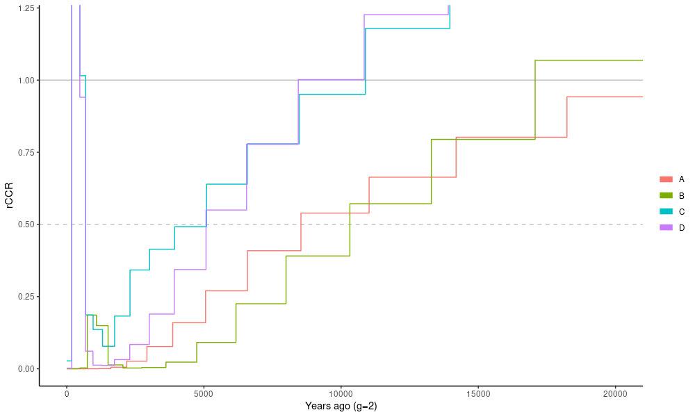
We see that the input files have one rate (lambda) whereas the combined output have three rates, two within the populations (00, 11) and one across (01). The relative cross-population coalescence rate is the ratio of these, more specifically \(2\lambda_{01}/(\lambda_{00}+\lambda_{11})\).

Again, this needs to be repeated with other population pairs. We do additional three pairs:

$ msmc2 -s -I 4-12,4-13,4-14,4-15,5-12,5-13,5-14,5-15,6-12,6-13,6-14,6-15,7-12,7-13,7-14,7-15 -o output/FINRYT_RUSLEV_LG3 multi/LG3.multihetsep.txt &> output/FINRYT_RUSLEV_LG3.runlog

$ msmc2 -s -I 8-12,8-13,8-14,8-15,9-12,9-13,9-14,9-15,10-12,10-13,10-14,10-15,11-12,11-13,11-14,11-15 -o output/RUSKRU_RUSLEV_LG3 multi/LG3.multihetsep.txt &> output/RUSKRU_RUSLEV_LG3.runlog

$ msmc2 -s -I 12-16,12-17,12-18,12-19,13-16,13-17,13-18,13-19,14-16,14-17,14-18,14-19,15-16,15-17,15-18,15-19 -o output/RUSLEV_RUSMAS_LG3 multi/LG3.multihetsep.txt &> output/RUSLEV_RUSMAS_LG3.runlog

These can then all be combined with:

$ echo FINRYT RUSLEV RUSKRU RUSLEV RUSLEV RUSMAS | xargs -n2 | while read pop1 pop2; do 
  $combinecc output/${pop1}_${pop2}_LG3.final.txt output/${pop1}_LG3.final.txt output/${pop2}_LG3.final.txt \
   > output/${pop1}_${pop2}_LG3.combined.msmc2.final.txt
done

Once these are computed, we can plot the results:

pairs <- c("FINKAR_FINRYT","FINRYT_RUSLEV","RUSKRU_RUSLEV","RUSLEV_RUSMAS")

# read in and combine the data 
dat.ccr <- c()
for(p in pairs) {
  tmp <- read.table(paste0("output/",p,"_LG3.combined.msmc2.final.txt"),head=T)
  dat.ccr <- rbind.data.frame(
    dat.ccr,
    cbind.data.frame(pair=p,tmp)
  )
}

# convert time boundaries to years and name coalescence rate ratio as ccr 
dat.ccr <- dat.ccr %>% mutate(time=left_time_boundary/mu*gt,ccr=2*lambda_01/(lambda_00+lambda_11))


ggplot(dat.ccr)+
  geom_hline(yintercept = c(0.5,1),color="gray",linetype=c("dashed","solid"))+
  geom_step(aes(x=time,y=ccr,group=pair,col=pair))+
  theme_classic()+ coord_cartesian(xlim=c(0,2e4),ylim=c(0,1.2)) + 
  xlab("Years ago (g=2)") + ylab("rCCR")

The result is slightly unorthodox and we would have assumed that the rCCR line is steadily increasing until it reaches 1, not going much over that. Probably our data set is too small for this and the analysis would be more robust with all the chromosomes. It is also notable that our data are not phased.

Traditionally, the time point where rCCR reaches 50% (dashed line) is considered the populations’ split time. We can indeed see that geographical distance between the populations correlates with their split times.

Exercise: Population split time with MSMC2

The figure below shows the relative cross-population coalescence rate (rCCR; y-axis) across time (x-axis) with the population labels hidden. Compare that to your plot and answer the questions in Moodle. When analysing the plot, ignore the spikes close to x=0 and focus on the part showing consistent increase on the y-axis.

rCCR plot.

Exercise 2 in Moodle.

MSMC-IM

The latest addition to MSMC2 methods is MSMC-IM that fits a continuous Isolation-Migration(IM) model to the estimates generated with MSMC2 and rCCR analysis. As it only requires the “*combined.msmc2.final.txt” files generated above, it is really quick to run. In my opinion, the improvements over MSMC2 and rCCR are highly significant.

The command requires the mutation rate that we have previously only provided in the plotting stage as well as the -beta parameter that we define as is recommended:

$ module load python-data

$ msmc_im=/projappl/project_2000598/sw/MSMC-IM/MSMC_IM.py 

$ $msmc_im -beta 1e-8,1e-6 -mu 1.42e-8 -o output/FINKAR_FINRYT_LG3 output/FINKAR_FINRYT_LG3.combined.msmc2.final.txt 

We can replicate the same for the three other population pairs as this:

$ for pair in FINRYT_RUSLEV RUSKRU_RUSLEV RUSLEV_RUSMAS; do
    $msmc_im -beta 1e-8,1e-6 -mu 1.42e-8 -o output/${pair}_LG3 output/${pair}_LG3.combined.msmc2.final.txt
done

(The commands may give warnings but they shouldn’t be too serious.)

Once this is finished, we can plot many things. The commands below are unnecessarily complex and include lots of formatting to make the plots look nice. I tend to spend long time fine-tuning the plots and try to make publication ready within R. I believe that this saves time in the long-run and sets the threshold for reanalysing the data (e.g. with different sample sets) very low.

As the first, we replot the effective population sizes across the time:

# read in and combine the data
dat.im <- c()
for(file in dir("output/","*MSMC_IM.estimates.txt")){
  tmp <- read.table(paste0("output/",file),head=T)
  pair <- substr(file,1,13)
  sp1 <- substr(file,1,6)
  sp2 <- substr(file,8,13)
  tmp$pair <- pair
  tmp$sp1 <- sp1
  tmp$sp2 <- sp2
  tmp$right_time_boundary = c(tmp$left_time_boundary[2:length(tmp$left_time_boundary)],Inf)
  dat.im <- rbind.data.frame(dat.im,tmp)
}
# cut 'm' at 0.999 
dat.im$m_prime <- if_else(dat.im$M <= 0.999, dat.im$m, 1e-30)

# plot the data
ggplot(dat.im) + 
  geom_line(aes(gt*left_time_boundary,im_N1,group=pair,color=sp1)) +
  geom_line(aes(gt*left_time_boundary,im_N2,group=pair,color=sp2)) +
  coord_cartesian(ylim=c(0,5e4)) + xlab("Years ago (g=2)") + ylab("Ne (mu=1.42e-8)") +
  theme_classic()+
  guides(color=guide_legend(title="",nrow = 1,override.aes=list(linewidth=3)))+
  theme(legend.key.width = unit(3,"mm"))+
  theme(text = element_text(size=8),
        axis.text = element_text(size=8),
        legend.position="top",
        legend.text = element_text(margin = margin(r = 3, l=1, unit = "pt"),size=9)
  )+
  scale_x_log10(
    minor_breaks = c(seq(1e3,10e3,1e3),seq(1e4,10e4,1e4),seq(1e5,10e5,1e5)),
    breaks=c(1e4,1e5),
    labels=c("10,000","100,000"),
    guide = "axis_minor",
    limits = c(500,5e5)
  )

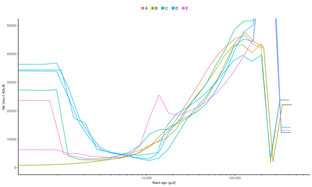
Compare this plot to the first MSMC2 plot: the two should show the same information.

There are now multiple estimates for the populations that were included in different cross-population comparisons. The different estimates (shown in population specific colours) are very consistent.

Exercise: Demographic history with MSMC-IM

The figure below shows the \(N_e\) (y-axis) trajectories across time (x-axis) with the population labels hidden. Compare that to your plot and answer the questions in Moodle.

Ne with MSMC-IM.

Exercise 3 in Moodle.

The second parameter of interest is m, the migration rate across time. This is best plotted with a function that can be replicated for different population pairs:

# convert time boundaries to years and subset columns
dat.m <- dat.im %>% select(left_time_boundary,m_prime,pair) %>% 
  mutate(time=gt*left_time_boundary) 

# colour-blind-friendly colours
cols <- palette.colors(palette = "Okabe-Ito")[c(7,4,8,6)]

plot_one <- function(df,cn,name) {
  ggplot(df) + 
    geom_step(aes(time,m_prime,group=pair),color=cols[cn]) +
    geom_rect(aes(xmin = time, xmax = lead(time), ymin = 0, ymax = m_prime,group=pair),
              color=cols[cn],fill=cols[cn], alpha = 0.1,linewidth=0.25) +
    scale_x_log10(
      minor_breaks = c(seq(1e3,10e3,1e3),seq(1e4,10e4,1e4),seq(1e5,10e5,1e5),seq(1e6,10e6,1e6)),
      breaks=c(1e3,1e4,1e5,1e6),
      labels=c("1,000","10,000","100,000","1,000,000"),
      guide = "axis_minor", # this is added to the original code
      limits = c(1000,1.15e6)
    )+
    theme_classic()+ theme(
      text = element_text(size=8),
      axis.text = element_text(size=8)
    ) +
    xlab("Years ago (g=10)") +  ylab("m_prime") + ylim(0,1.7e-4) +
    annotate("text", x=1000,y=1.6e-4,label=name,size=3,hjust = 0, )
}

pl.m1 <- plot_one(subset(dat.m,pair=="FINKAR_FINRYT"),1,"FINKAR_FINRYT")
pl.m2 <- plot_one(subset(dat.m,pair=="FINRYT_RUSLEV"),2,"FINRYT_RUSLEV")
pl.m3 <- plot_one(subset(dat.m,pair=="RUSKRU_RUSLEV"),3,"RUSKRU_RUSLEV")
pl.m4 <- plot_one(subset(dat.m,pair=="RUSLEV_RUSMAS"),4,"RUSLEV_RUSMAS")

plot_grid(pl.m1,pl.m2,pl.m3,pl.m4,ncol=1)

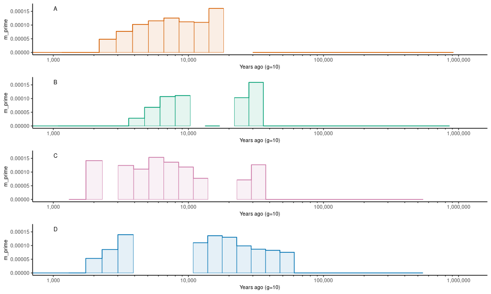
On this plot, we used m_prime that is cut at the point where M, the cumulative migration, reaches 0.999 and thus 99.9% of the information is used. The program produces estimates of m beyond that point but they are based on such minute changes in the relative coalescence rates that the output is mostly noise.

The estimates of migration (y-axis) contain strange gaps at some time ranges (x-axis) but generally the output appears consistent with the expected population histories.

Exercise: Population split time with MSMC-IM

The figure below shows the migration rates (m_prime; y-axis) across time (x-axis) with the population labels hidden. Compare that to your plot and answer the questions in Moodle.

Migration rates with MSMC-IM.

Exercise 4 in Moodle.

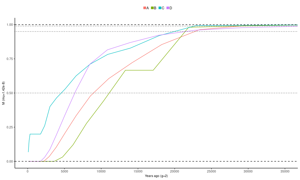
Finally, we plot M, the cumulative migration across time:

ggplot(dat.im) + 
  geom_line(aes(gt*right_time_boundary,M,group=pair,color=pair)) +
  geom_hline(yintercept = c(0,1),linetype="dashed") +
  geom_hline(yintercept = c(0.5,0.95,0.99),linetype="dotted") +
  coord_cartesian(xlim=c(1,3.5e4))+
  xlab("Years ago (g=2)") +  ylab("M (mu=1.42e-8)") + theme_classic()+
  scale_x_continuous(breaks=seq(0,35000,5000))+
  guides(color=guide_legend(title="",nrow = 1,override.aes=list(linewidth=3)))+
  theme(
    legend.key.width = unit(1,"mm"),
    text = element_text(size=8),
    axis.text = element_text(size=8),
    legend.position="top",
    legend.text = element_text(margin = margin(r = -1, l=0, unit = "pt"),size=9)
  )

Similarly to rCCR, the time points where M reaches a specific threshold (dotted lines) can be considered population split times. The 50% threshold is commonly used but also the higher threshold (95% and 99% are shown) can be of interest. Such as function is provided in Python as a part of the MSMC-IM package. We can port it to R and use it to compute the intersection points between M and an arbitrary threshold:

getCDFintersect <- function(t, CDF, val){
    xVec <- t
    yVec <- CDF
    i <- 1
    CDFintersect <- NaN
    if(yVec[1] < val){
        while(yVec[i] < val) {
            i <- i + 1
        }
        if(! i > 0 | ! i <= length(yVec)){ 
            print("CDF intersection index out of bounds: ",i)
        }
        if(! yVec[i - 1] < val | ! yVec[i] >= val){
            print("this should never happen")
        }
        intersectDistance <- (val - yVec[i - 1]) / (yVec[i] - yVec[i - 1])
        CDFintersect = xVec[i - 1] + intersectDistance * (xVec[i] - xVec[i - 1])
    } else {
        CDFintersect <- val/yVec[1] * xVec[1]
    }
    return (CDFintersect)
}
  
dat.im %>% group_by(pair) %>% 
    reframe(pair,
            x50=getCDFintersect(gt*right_time_boundary, M, 0.5),
            x95=getCDFintersect(gt*right_time_boundary, M, 0.95)
    ) %>% distinct()   

With that, one can calculate the exact time points where the lines cross.

Exercise: Cumulative migration with MSMC-IM

The figure below shows the cumulative migration (M; y-axis) across time (x-axis) with the population labels hidden. Compare that to your plot and answer the questions in Moodle.

‘M’ with MSMC-IM.

Exercise 5 in Moodle.

Conservation genetics of Saimaa ringed seals

The analyses of the Saimaa ringed population analysis are described in detail in a STAR Protocols article. The code is available in a GitHub repository, allowing reproduction of the analyses with a subset of data. We do not replicate the analyses here but those interested in the concepts are welcome study the documentation in detail and reproduce the results by themselves.

The code is provided as bash, awk and R scripts as well as Jupyter notebooks. Unfortunately, GitHub doesn’t show the notebooks correctly; one solution is to use an external notebook viewer to show the code. To do that, one should click the “Raw” button to open the “raw” code in GitHub:

and then copy the URL address of the file (starting with “https://raw.githubusercontent.com/”) and paste that to https://ipynb.js.org/. This then shows the notebook with the correct formatting.

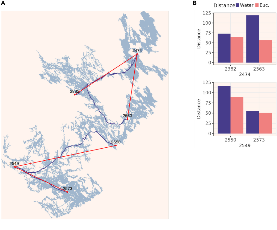
This particular notebook may be of use beyond population genetic studies and contains the R code to compute the water distances between geographic coordinates using a map downloaded from the Finnish Environment Institute open data service. When studying aquatic organisms, it is good to notice the water distances may differ from the straight Euclidean distance:

Difference between water and Euclidean distances.

Take-home message

The coalescence model provides a framework to estimate the effective population size from sequence data. Sequential Markov models have become popular in inferences of demographic histories of populations and divergence times between populations. MSMC2 is the latest version of the approach started by PSMC and can be used for inferences from one or several diploid genomes. MSMC2 infers the cross-over breakpoints in the genome using a HMM, computes the distribution of coalescence times and then fits this distribution to a model of segmented time, the population size possibly varying between the time segments.

By performing the coalescence analysis within two populations and between them, one can compute the relative cross-population coalescence rate and infer the split time between the populations. MSMC-IM is a related method that fits an Isolation-with-Migration model to the inferred coalescence rates: from that, one can obtain improved estimates of effective population sizes, an estimate of migration rate across time and the cumulative migration. The amount of information contained in the data depends on the population size and one cannot see deeper in the past than the data allow. Inferences of migration rate across time should be stopped at the point where the cumulative migration has reached 99.9%.

MSMC2 plot. rCCR plot. Ne with MSMC-IM. Migration rates with MSMC-IM. ‘M’ with MSMC-IM. Difference between water and Euclidean distances.