4. Wright-Fisher and coalescence theory

Learning outcome

After this chapter, the students can describe the concepts “Wright-Fisher population model” and “genetic drift” and explain the impact of population size on genetic drift. They can also explain how lineages “coalesce” in a W-F population and describe the expected shape of a multi-sample coalescence tree.

Wright-Fisher model and Drift

Population genetics studies distributions and changes of allele frequencies in populations over time. The effects considered include:

natural selection
genetic drift
mutation
gene flow
recombination
population subdivision

Population genetic methods allow inferring past events as well as predicting the future.

The fundamental work on modern population genetics was done by Haldane, Wright and Fisher on the first half of 20th century. A significant more recent development is the coalescent theory independently by Kingman, Hudon and Tajima in the 1980s. The coalescent theory is especially suitable for the SNP data and computationally highly efficient, making it the backbone of much of the modern analysis methods.

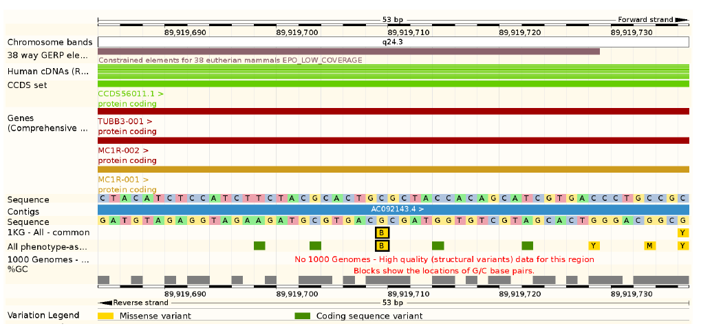
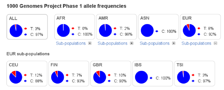
“Allele” is one of alternative forms of a gene or same genetic locus. It used to mean (and in some context may still mean) a visible gene product (e.g. blond vs. red hair) but we now typically refer alleles at SNP positions (e.g. rs1805007(C) vs. rs1805007(T))

Alleles in a genetic locus do not need to be functional and, in many studies, the expectation is that the variation is neutral, i.e. its evolution and changes in allele frequencies ahave not been affected by selection. Above, the SNP in Melanocortin_1 receptor affects the hair colour; in addition, the SNP “rs1805007” is associated e.g. with “Skin sensitivity to sun”, “Non-melanoma skin cancer” and “Freckles”. In some conditions, the alleles are probably under selection. However, genomes provide millions of variable loci, and a majority of those are thought to be neutral.

Wright-Fisher population model

Mathematical models of population evolution cannot taken into account all the complexities of biological life and assume a simplified population. The most commonly used population model is the Wright-Fisher model. It assumes e.g.:

haploid population
no sex
constant population size

Very few natural population is even close to that. The Wright-Fisher model (WFM) can be generalised e.g. for diploid population with random mating and for variable population size, but even these assumptions are typically too stringent for natural populations.

We do not need to believe that the target population follows the WFM for the model to be useful. Even if the target populations are more complex populations than the WFM, the model can give a good approximation for their evolution and allow comparing different populations.

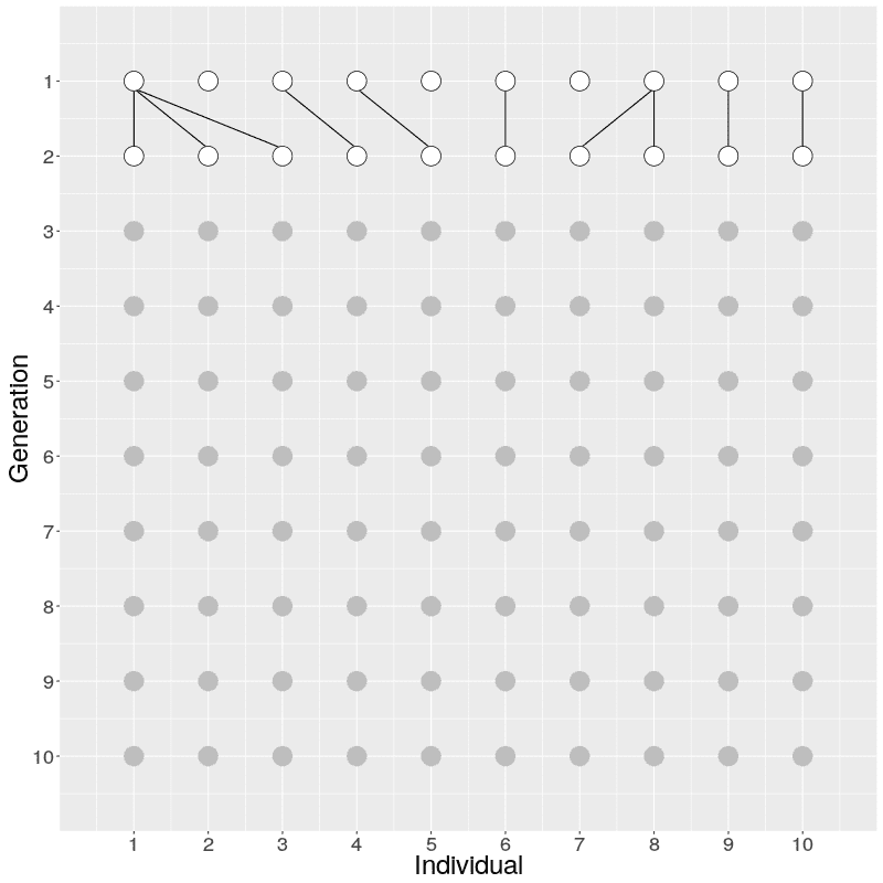
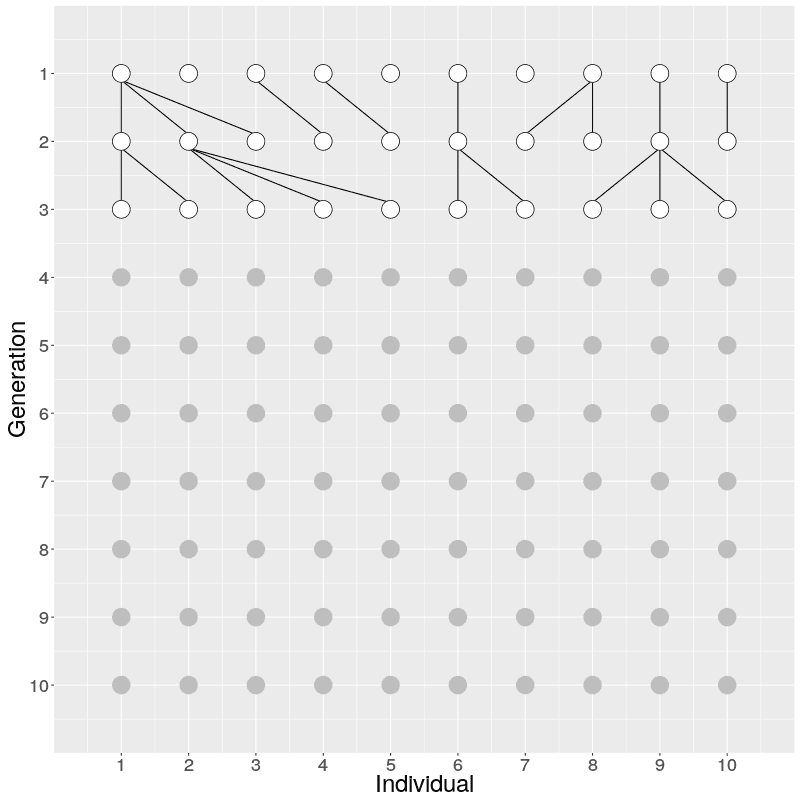
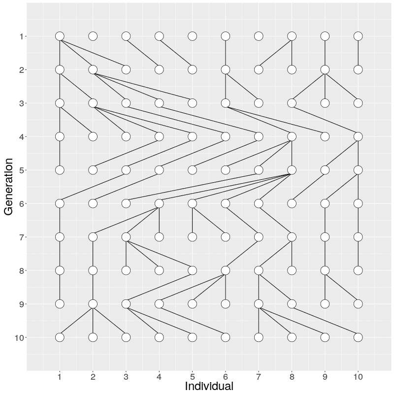
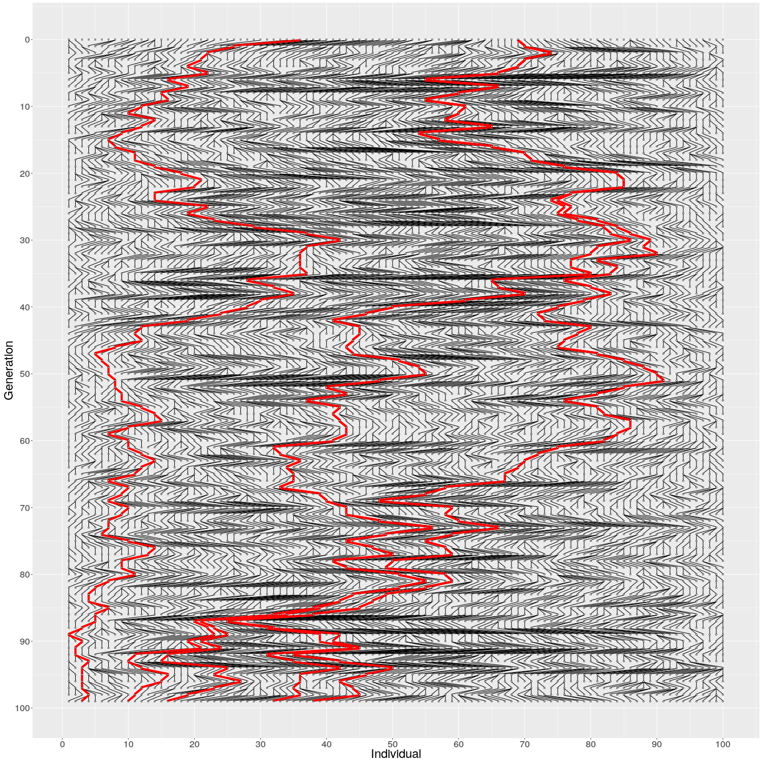
The evolution of 10 individuals (on x axis) over 10 generations (on y axis) can look like this:

On Generation 1, we have 10 individuals. The individuals on Generation 2 are created by randomly sampling the parent for each from Generation 1; because of this randomness, some individuals on Generation 1 have multiple offspring while others have none. The individuals on Generation 3 are similarly created by randomly sampling the parents from Generation 2. This is continued until Generation 10.

When we look at the realisation of the evolution over ten generations, we can see two things:

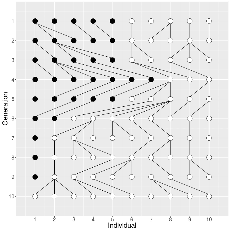
If the individuals in Generation 1 would have carried two alleles, a half black and another half white, the frequency of the alleles changes over the generations (in middle) and the black allele disappears, leading the white allele in fixation. The alleles cannot reappear (without migration or mutation that we do not allow here) meaning that the red black is lost forever. The random change in allele frequencies is called genetic drift.

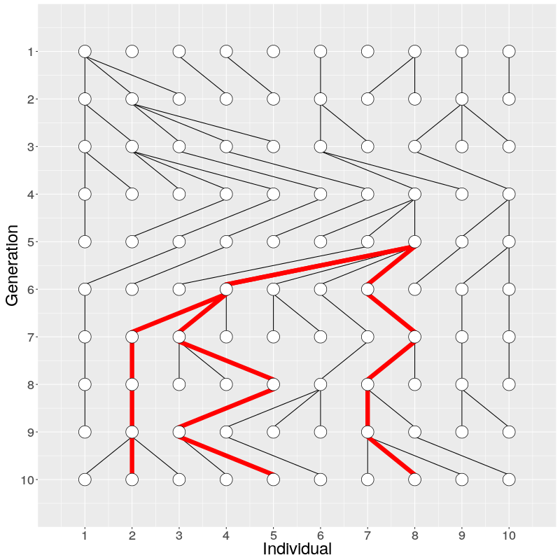
In the figure on the right, three individuals on Generation 10 are selected and the links to their parents and ancestors are tracked backwards. We notice that the lineage merge – or coalesce – on Generation 5, all three lineages have joined and we have reached the Most Recent Common Ancestor (MRCA). This joining of lineages is called coalescence process.

Genetic drift

Allele frequencies change by chance from one generation to the next, the size of change per generation depending on \(N_e\), the effective population size. At every locus, variation is eventually lost and one allele becomes fixed:

at non-neutral loci, selection affects chances of fixation
variation is lost much more rapidly in small populations
in small populations genetic drift can prevail selection and even harmful alleles may get fixed

Variation once lost is lost forever

population bottleneck reduces variation
population recovery cannot bring it back
new variation is created by mutations

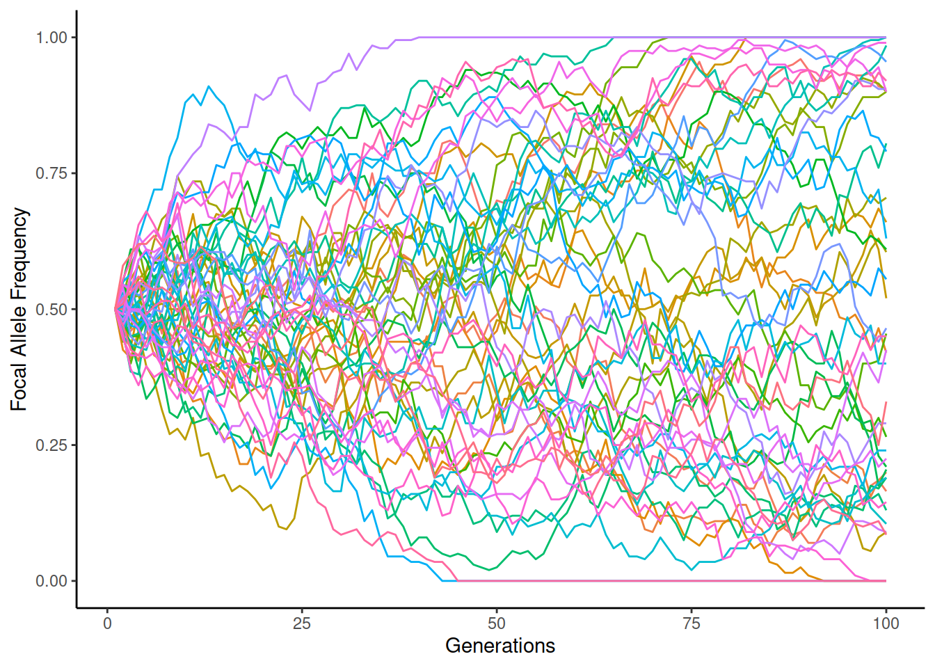
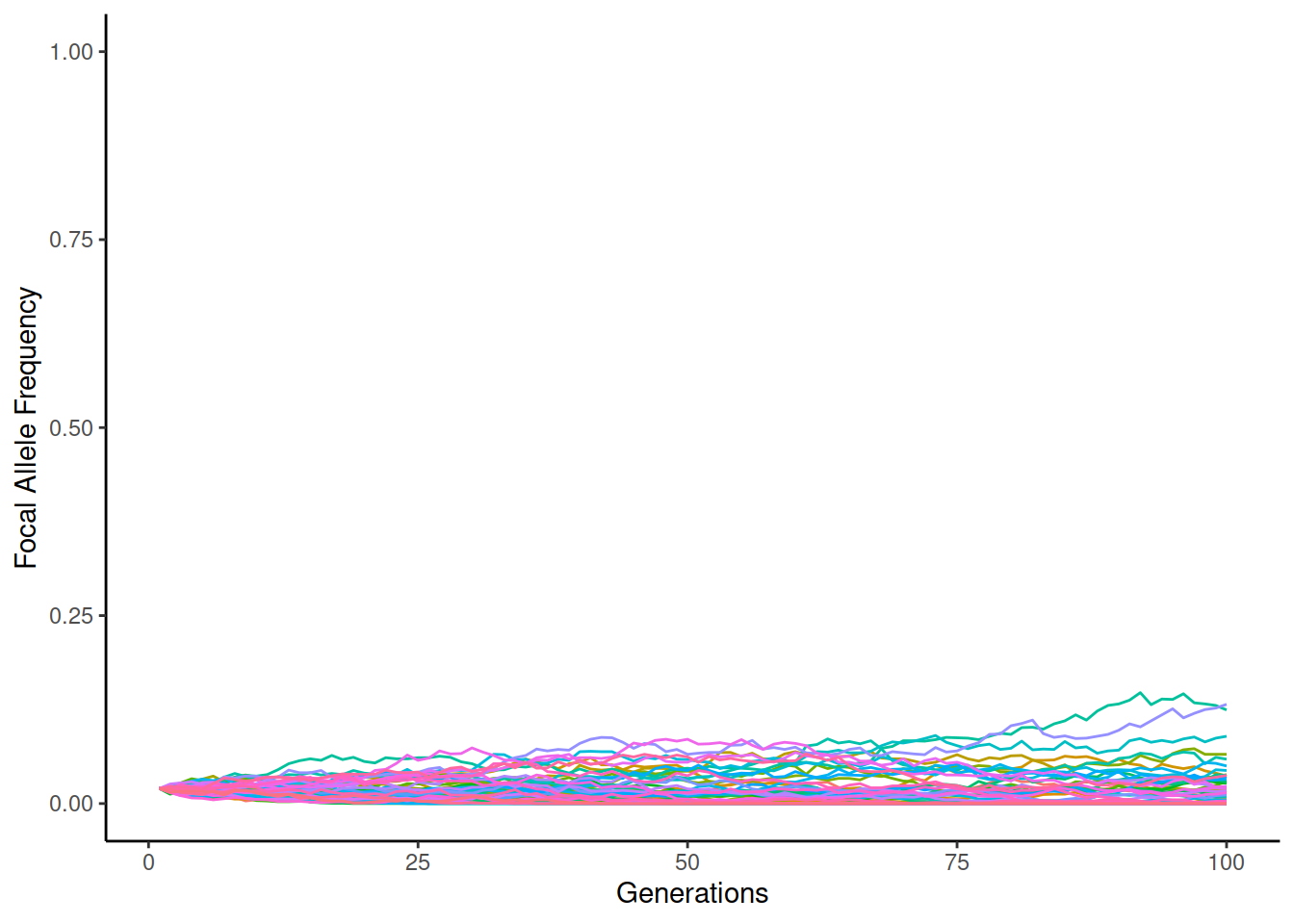
We can easily simulate evolution under WFM. Below, the lines show the allele frequency in different simulation replicates (in total 50), each replicate shown in different colour. The initial frequency of the focal allele is 50% and it may go up or down over the generations; if the frequency reaches 0 or 1, one of the alleles becomes fixed and the frequency cannot change any more. On the left, \(N_e=2000\), on the right \(N_e=200\):

We can see that the drift is much greater in the smaller population and some of the replicates become fixed to one of the alleles when \(N_e=200\).

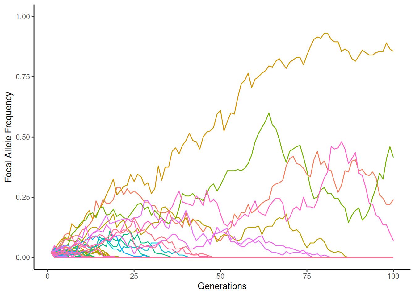
On the other hand, in small populations, the chances of rapid changes in allele frequency are possible. When the starting frequency is just 2%, the simulation may look like this:

The two alleles stay more frequently alive when \(N_e=2000\) but the frequency of individual replicates increases to the highest values when \(N_e=200\). However, in the latter case, a great majority of replicates go to zero and become fixed to one allele.

Simulating genetic drift

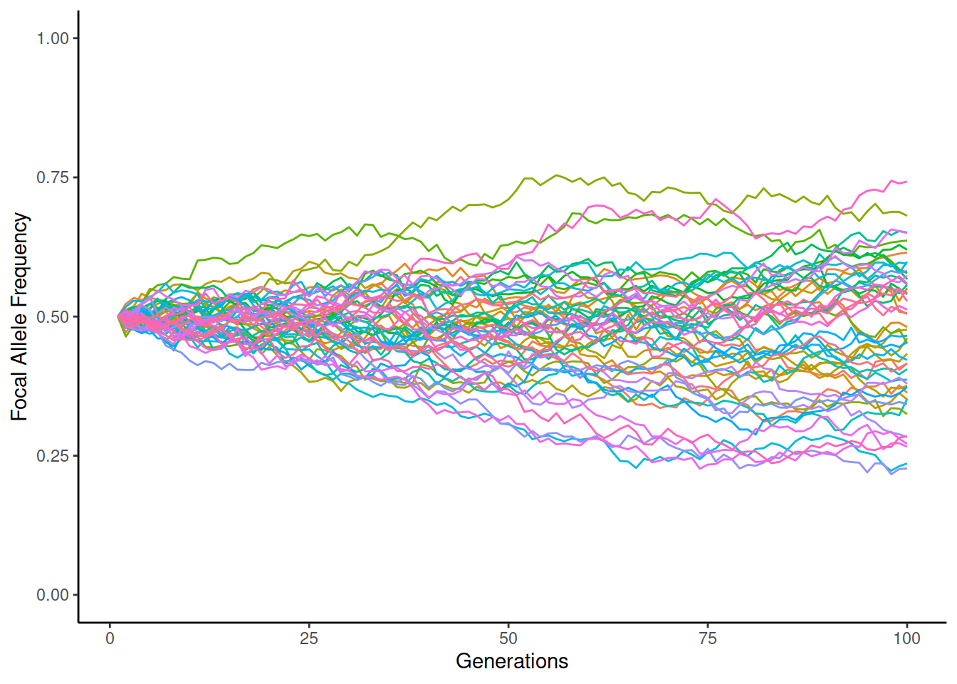
You can test how the strength of genetic drift (change in allele frequency on the y-axis) depends on the population size. Below, the allele frequencies are simulated over 100 generations (x-axis) for 50 replicates (lines with different colours). The initial allele frequency affects the chances of fixation (numbers on the right).

Try setting the allele frequency at 0.50 and population size at 50 and see how the number of fixed runs is distributed between 0 and 1. Repeat the simulation multiple times. Try then changing the allele frequency (e.g. at 0.4 or 0.6) and test how this affects the numbers.
Try setting the allele frequency at 0.01 and population size at 50 and simulate new runs until you see the allele frequency fixing to 1. This seems unlikely but can easily happen.
Try setting the population size at 5000 and allele frequency at a low value and see if any runs get fixed.

\(N_e\), the effective population size

Even if the target populations wouldn’t fulfil the assumptions of the WFM, the model can provide useful estimates. One of the central estimates in population genetics is the size of the population. For some populations or species, we may have estimates of \(N_c\), the census size (e.g. there are decent estimates of the number of wolves in Finland and rather precise estimates of the number of ringed seals in lake Saimaa), but those are based on counting, not population genetic analyses. With genetic data, we can estimate \(N_e\), the effective size of the population. In the context of WFM, \(N_e\) is the size of WFM population that genetically behaves in a similar manner to the target population.

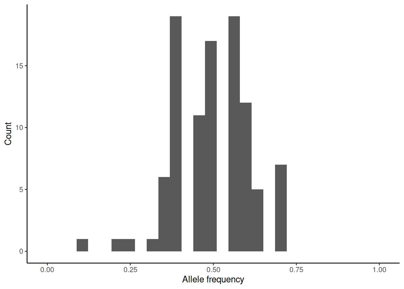
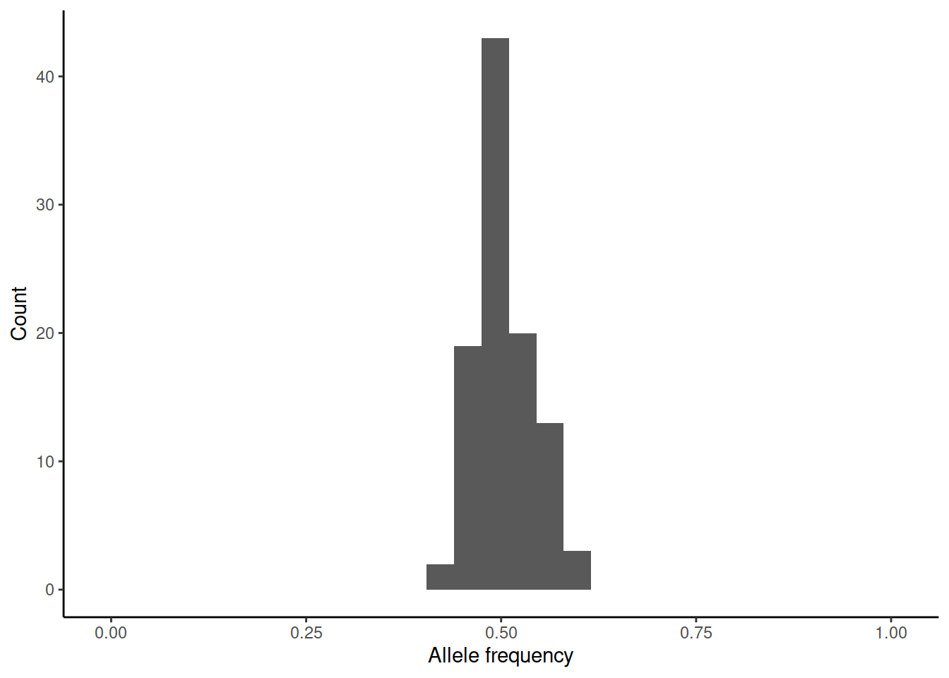
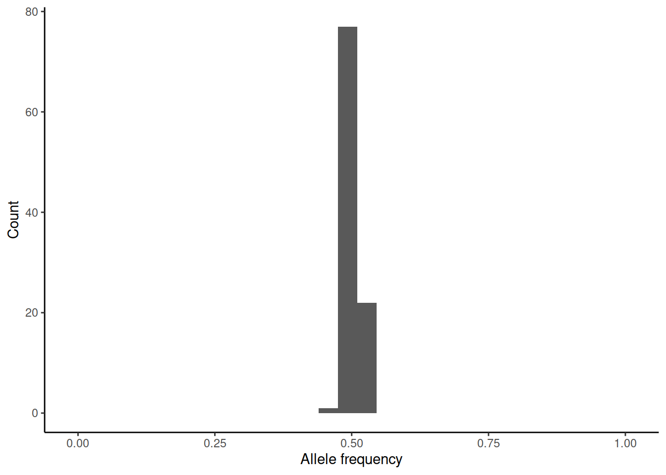
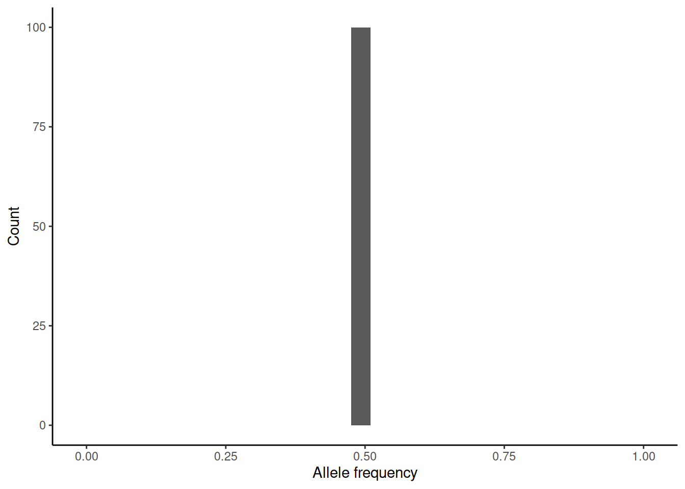
This brings us back to genetic drift. One way of measuring \(N_e\) is to estimate the variance of allele frequency change per generation. We can again simulate (rbinom(100,n,0.5)/n) how the initial allele frequency of 0.5 would change over one generation in differently sized populations:

In practice, the estimation of the variance is difficult as accurate estimates of allele frequencies require large sample sizes and these should be done on subsequent generations.

However, in addition to changes in allele frequencies, the drift can be also looked in the context of the coalescence process. There, small populations coalesce faster and have a more recent MRCA:

That concept – or rather its inverse – is widely used in population genetic analyses: \(N_e\) can be defined as a function of the coalescence time. If all the lineages coalesce quickly, the population has a small \(N_e\); if they coalesce slowly (MRCA is in the deep past), the population has a large \(N_e\).

It is notable \(N_e\) is not the same as \(N_c\), the census size of a population, and the two can be vastly different from each other. There can be many reasons for a distant MRCA – e.g. population structure and migration among the sub-populations – but they nevertheless increase the coalescent \(N_e\). If the MRCA is distant, the Wright-Fisher population producing a similar coalescence process has to be large.

Wright-Fisher model and Coalescence

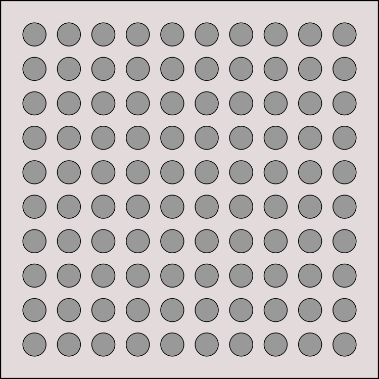
Let’s assume that we have two marble balls (\(\bullet \bullet\)) and a sieve like this:

How many times do we have to throw the balls for them to fall in the same hole?

We can break this into two parts:

first ball can fall anywhere
second ball falls in the same hole with the probability \(1/N\) (where \(N\) is the number of holes)

Now, let’s assume a population with \(N\) individuals and two samples.

how many generations we have to go back for them to coalesce?

first sample can have any parent

second sample has the same parent with the probability \(1/N\)
second sample has a different parent with the probability \(1-1/N\)

If the two samples have different parents at generation -1, this continues to generation -2:

The lineages may coalesce:

or continue as separate lineages:

Probability of coalescence on generation \(r\) before present follows geometric distribution: \((1 − 1/(N))^{r −1} 1/(N)\)

Coalescence process is memoryless and the waiting time for the next event is not affected by past failures
The mean of geometric distribution with probability \(p\) is \(1/p\). For \(p=1/N\) that is \(1/(1/N)\) or \(N\)
For example, for \(N=40\), the expected time for two random lineages to coalesce is 40 generations
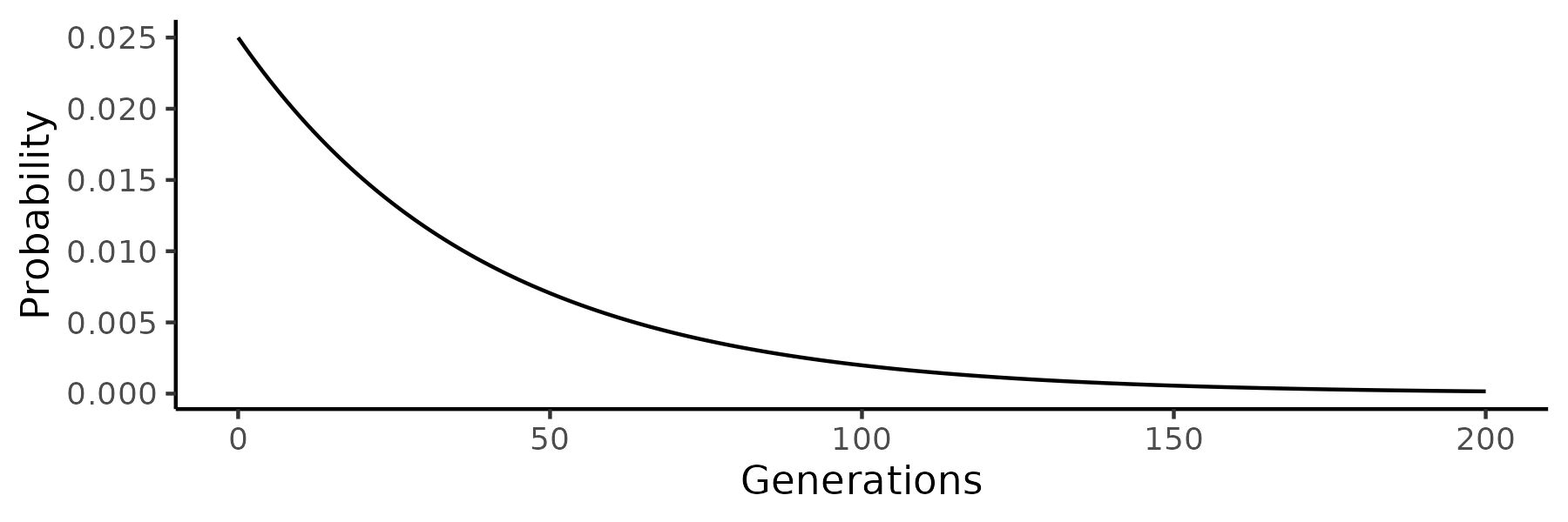
Of individual coalescence times, the greatest probability is for generation 1 but the tail is very long (this is for \(N=40\)):

When \(p\) gets very small, geometric distribution converges to exponential distribution: \[ \lim_{n\rightarrow\infty} \left(1 - \frac{\alpha}{n}\right)^n = e^{-\alpha} \]

For large \(N\), the coalescence process follows an exponential distribution.

Important

Confusingly, some population genetics text books talk about \(N\) individuals (with \(N\) chromosomes or sequences) and some others of \(N\) diploid organisms with \(2N\) chromosomes. Here, we assume the former such that the population size, that is the number of chromosomes, is \(N\).

Coalescence of many lineages

Now let’s assume that we have a sieve and five marble balls (\(\bullet \bullet \bullet \bullet \bullet\)):

How many times do we have to throw the balls for them to fall in the same hole?

As above, we can convert this to a population with N individuals and five samples:

how many generations we have to go back for them to coalesce?

first sample can have any parent

second sample has the same parent with the probability \(1/N\)
second sample has a different parent with the probability \(1-1/N\)

If different,

third sample has the same parent with the probability \(2/N\)
third sample has a different parent with the probability \(1-2/N\)

If different,

fourth sample has the same parent with the probability \(3/N\)
fourth sample has a different parent with the probability \(1-3/N\)

If different,

fifth sample has the same parent with the probability \(4/N\)
fifth sample has a different parent with the probability \(1-4/N\)

For \(n\) lineages, coalescence rate is \((n(n − 1)/2)(1/N)\) (assuming large \(N\))

for \(N = 40\), the coalescent rate and the expected time (in generations) to the next event are:

Lineages	Rate	Time
5	0.25	4
4	0.15	6.67
3	0.075	13.33
2	0.025	40
total		64

when \(n\) is large, coalescent events happen quickly
last event (\(n = 2\)) is expected to take at least half of total time

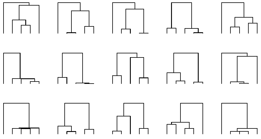
Expected coalescence times have large variance, tree shapes differ greatly:

Note that WFM allows one parent to produce more than two offspring, meaning that more than two lineages may coalesce in the same generation. For large \(N\), the chances of two or more events in a generation are tiny and the process simplifies to coalescence of two lineages at a time:

Important

It is crucial to see the differences between phylogenetic and population genetic analyses. In phylogenetic analyses:

sequences of different divergence levels
observed differences allow inferring tree of evolutionary relationships

whereas in population genetic analyses:

observed sequences can be identical
coalescent theory proves that sequences are related by a tree
often the tree shape cannot be inferred
many properties of the tree are known even without any sequence data!
genealogy (family history) often considered a nuisance parameter

Take-home message

Natural populations are far too complex for many mathematical analyses and typically a highly simplified model of a population is used. The most widely of these is the Wright-Fisher population model, devised independently by Sewall Wright and Ronald Fisher in the early 20th century. Population genetics studies changes in allele frequencies. On this course, we largely focus on neutral evolution and allele frequency changes caused by genetic drift. The drift is the greatest in small populations and can be negligible in very large populations.

In a WFM population, some lineages die out and some parents produce multiple offspring. When tracking back multiple lineages, the lineages join – or coalesce. The properties of this coalescence process is the key information for many modern inference methods.

The basic mathematics of coalescence theory is fairly simple. A key property is that, in an analysis of multiple samples, the first coalescence events happen quickly and the last even, between the last two remaining lineages, is expected to take the most time. The variance is great, however.