1. Puhti and a glimpse on a reference genome

Learning outcome

After this practical, the students recognise the file formats used for reference genomes, gene annotations and region masks and an find information in them using an index. They can describe the relation between text-formatted raw-data and the illustration of the data in a graphical genome browser.

Using the course machine on Puhti

The exercises are done on CSC Puhti supercomputer under the project “2000598”. You got the membership to this project on the course EEB-021. If you are not a member, please see the Moodle page for instructions on how to apply for membership.

The practicals can be done using (i) a stand-alone terminal program or (ii) the shell terminal through a web browser.

Stand-alone terminal

Every Linux-user should know what is “Terminal” and be able to open it (if not, search for the term “terminal” and start that program). Instructions for Windows and MacOS are provided at https://intscicom.biocenter.helsinki.fi/section10.html.

With a terminal program, you can open a connection to Puhti, providing the password when asked, with SSH as:

$ ssh username@puhti.csc.fi

[username@puhti-login12 ~]$

Syntax of the code boxes

The commands start with a dollar sign ($) and can be multiple lines long. You should write or copy-paste the full command in your terminal and then execute it by pressing Enter. Sometimes another code box is shown with the output of the command. This does not start with a dollar sign and should not be executed.

This command brings you to one of the “login nodes” of Puhti (there are multiple and yours can be different from “puhti-login12” shown above). The second last character before the prompt symbol (“~”) indicates that you are in the home directory.

On Puhti, home directories are small in size and you should not do your analyses there. Instead, the actual space-demanding and computation-heavy work should be done under /scratch/project_2000598/. For simplicity, we call that “$WORK”. Make first a directory named by username and go that directory:

$ WORK=/scratch/project_2000598
$ mkdir $WORK/$USER
$ cd $WORK/$USER

Why is it called scratch?

If not limited, we all quickly fill up the available storage space (on a laptop, mobile phone etc.) with (copies of) documents and files that are not truly necessary or that should be organised and collected in a more formal way. That is also a problem on CSC supercomputers and they need to limit the use of disk space somehow. One of their rules is that they may delete files that have not been accessed for six months. This rule is applied to files under /scratch.

In scientific analysis, one can live with that rule. If the analyses continue and the files are regularly accessed, they won’t be deleted. If the analyses have finished, the necessary files (e.g. the raw data, analysis scripts and final results; see https://intscicom.biocenter.helsinki.fi/section9.html) should be moved elsewhere and archived in a more structured form.

This course takes less than two months and the rule won’t affect the course works. If you want to store some of the files for later, you should copy them elsewhere.

As mentioned earlier, you get to Puhti through a login node but that node (=a computer with 20 cores) is not meant for heavy computing. Instead, the work should be done using the SLURM job scheduler that shares the (limited) resources in a fair manner. The use of batch jobs is explained at https://intscicom.biocenter.helsinki.fi/section5.html#running-jobs-on-a-linux-cluster.

Many of the tasks on this course can be done interactively. The basics of interactive SLURM jobs is explained at https://intscicom.biocenter.helsinki.fi/section5.html#example-interactive-job.

An interactive session for 6:00 hours with 4 GB (=4000 MB) of memory and 1 computation core can be started with:

$ sinteractive --account project_2000598 --time 6:00:00 --mem 4000 --cores 1

[username@r18c03 username]$

This now created a bash terminal on computation node r18c03 (yours can be different).

You can close the terminal with logout or Ctrl+d. If not closed earlier, the terminal job will expire after six hours. All the work and files finished before the expiration will be retained and can be seen in their locations in a terminal on a login node or in another interactive terminal.

Terminal through a web browser

Accessing Puhti through a web browser is explained at https://intscicom.biocenter.helsinki.fi/section0.html#registration-and-access-to-the-course-machine and the web-based terminal is explained at https://intscicom.biocenter.helsinki.fi/section0.html#alternative-terminal.

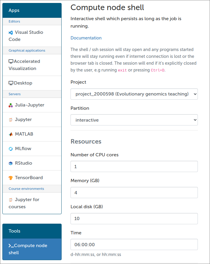
In brief, the tools menu contains “Login node shell” and “Compute node shell”:

The “Login node shell” is identical to a SSH access to a Puhti login node. One can enter Puhti through that and then start an interactive job as explained above. Choosing “Compute node shell” basically does the sinteractive command and directly opens a terminal on a compute node.

For “Compute node shell”, these settings create a session for 6:00 hours with 4 GB (=4000 MB) of memory and 1 computation core:

Other tools on Puhti

Even when using a stand-alone terminal program, it may be useful to login to https://www.puhti.csc.fi/public/ and use the web tools there. I personally use a combination of vi (explained here https://intscicom.biocenter.helsinki.fi/section5.html#text-editing-in-the-command-line) and the text editor within Jupyter (explained here https://intscicom.biocenter.helsinki.fi/section5.html#text-editor-within-jupyter) when working on Puhti. For a beginner, the Jupyter text editor is highly recommended. If necessary, rehearse how to start a Jupyter session from https://intscicom.biocenter.helsinki.fi/section0.html#different-options-for-doing-the-course-exercises. Note that you can select the regular “Jupyter” instead of “Jupyter for courses”.

Jupyter can be used as a file browser and visualisation tool, but the file system, including the /scratch space, can also be seen under “Files” on the Puhti web interface (in the top panel):

Through this, one can navigate in the filesystem, open files (in a supported format, e.g. graphics and text) inside the web browser, download the files to one’s own computer or upload local files to Puhti:

Transferring files to/from Puhti on command line

In addition to the web interface, files can be moved back and forth using command-line tools. The most important of these is the command scp [from] [to] that uses the SSH protocol. Typically, the scp command has to be performed on one’s own computer (inside a terminal program).

A local file can be copied to Puhti with the command:

$ scp local_file.txt username@puhti.csc.fi:/scratch/project_2000598/username/data/

A remote file can be copied to one’s own computer with the command:

$ scp username@puhti.csc.fi:/scratch/project_2000598/username/data/remote_file.txt .

Here, the dot in the end means “here”.

In the scp command, the remote file path consists of user (username), computer (puhti.csc.fi) and file path (/scratch/project_2000598/username/data/remote_file.txt). The first two are separated by @ and the last two by :. On Puhti, the absolute file path of the file “remote_file.txt” can be obtained with the command

$ readlink -m remote_file.txt

SSH key makes the work on a stand-alone terminal easier

The SSH protocol encrypts the traffic between your own computer and the target computer such that the possible listeners cannot see what you are doing (ssh) or what kind of data you are transferring (scp). The commands need authentication every time they are started, possibly making the use of scp command painful.

Those working a lots on remote Linux servers should learn to use SSH keys. The concept of keys is explained at https://intscicom.biocenter.helsinki.fi/section9.html#public-private-key-authentication.

To set up an SSH key on Puhti, one needs to

Generate a key pair on one’s local computer
Copy the public key to Puhti
Append the public key in the end of file ~/.ssh/known_hosts.

If the directory ~/.ssh doesn’t exist, create it and set it readable by you only:

$ mkdir ~/.ssh
$ chmod go-rwx ~/.ssh

The file ~/.ssh/known_hosts may contain public keys of many computers (and thus allowing access from each without password authentication) and you should not overwrite but append it. If the file doesn’t exist, create one.

If successful, you can now open an ssh connection (ssh username@puhti.csc.fi) or copy files (scp [from] [to]) without providing the password. The authentication is done using the public/private key pair by the SSH protocol.

When done correctly, this is fully secure. Remember that you should never share or copy the private SSH key!

A reference genome

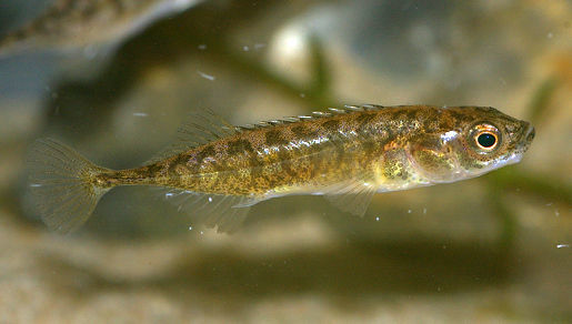
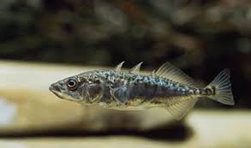
On this course, we work a lot with the nine-spined stickleback data. Nine-spined stickleback (Pungitius pungitius; Wikipedia) is a small, economically non-important fish that inhabits temperate waters. In Finland, it is found in coastal waters and numerous ponds, lakes, streams and rivers. Due to its ability to survive in nearly every environment, it has been studied at UH as an evolutionary genetics model of adaptation. Its (relatively distant) cousin, three-spined stickleback (Gasterosteus aculeatus; Wikipedia), is a globally known model species in ecology and evolutionary genomics.

The UH research group led by prof Juha Merilä (now in Hong Kong, China) has produced a reference genome for the ninespine. The reference genome has been upgraded multiple times (v5, v7, v8) but, for learning purposes, some of our analyses utilise the very first draft version. To be more precise, we utilise a small proportion of the full genome, 100 of the total 5280 contigs; this makes the analyses run faster and practical in the course settings.

A “contig” means a continuous fragment of a genome sequence produced by the assembly program. In the current age of HiFi sequencing, the “draft” assembly may consist of less than 100 contigs, meaning that nearly every chromosome arm has been assembled to one continuous piece of sequence. (Centromeres are often highly repetitive and it can be difficult to connect the two chromosome arms together with sequence information only.) In the age of short-read sequencing, genome assemblies often consisted of tens or even hundred of thousands of contigs. With the help of first-generation long-read sequencing, the number could be dropped to a few thousand contigs; the ninespine genome is from that period

Continuity of the reference genome and having the sequence as full chromosomes is not especially important for population genetic studies. More important is that the genome is largely “haploid”, meaning that each region of the genome – shared by the sister chromosomes inherited from the maternal and paternal sides – is represented only once. The difficulty is that some genome regions have duplicated, often known as “segmental duplications”, and in some parts of the genome, the maternal and paternal copies may differ significantly, creating distinct “haplotypes”. The original contig-level assembly contains segmental duplications and haplotypes as multiple fairly similar copies of a sequence. The challenge is to keep the segmental duplications but drop the haplotype copies when “scaffolding” the contigs into longer sequences. Technically, these longer sequences, “scaffolds”, are not complete and shown experimentally to belong together. Instead of calling them “chromosomes”, they are often called “linkage groups”, indicating that they appear to be associated and are inherited together.

FASTA and FASTA index

Make a copy of the reference genome:

$ WORK=/scratch/project_2000598
$ cd $WORK/$USER
$ mkdir reference
$ cp $WORK/shared/reference/ninespine.fa.gz reference/

The file is compressed and roughly 3 MB in size and looks like DNA:

$ ls -lh reference/ninespine.fa.gz

-rw-rw---- 1 username pepr_username 3.0M Sep 18 18:11 reference/ninespine.fa.gz

and

$ zcat reference/ninespine.fa.gz | head -4

>ctg7180000005484
CGTCACACTAACAGCTGCCCATCTGGTTACTGTCAGGGAGAAAACAACTGAGCTTGCGGA
GACTTTATGAGGTACTGGACTTACTGTATGTATGTATATATTTATATTCATCTAATGGGC
ATCTGTTTAACATAAAGTGATGCATTCAAGTTTTGTTTCAAAGCAGGGATGATCAAAGCT

This is the look of a FASTA-formatted sequence file. The format uses “>” as a marker of header lines that specify the name of the sequence below. In a genome file that could “>chr1”, “>chr2” and so on, or as here, the contig names. A FASTA file can contain one or many sequences. It is valid to write the sequence on one line only (this may then be wrapped up by the text viewer program or continue out of the window on the right) or to use newline characters to neatly place on rows of uniform length (with the exception of the last row).

As seen of the file suffix, this file is compressed. Many of the analyses tools could work with this compressed format but not all of them. We therefore decompress it. After that, we’ll create an index. For that we need to load the program samtools from the module “samtools”:

$ gunzip reference/ninespine.fa.gz
$ module load samtools
$ samtools faidx reference/ninespine.fa
$ head reference/ninespine.fa.fai

ctg7180000005484    697083  18  60  61
ctg7180000005545    816998  708738  60  61
ctg7180000005546    21996   1539371 60  61
ctg7180000005574    57200   1561752 60  61
ctg7180000005586    1225367 1619924 60  61
ctg7180000005587    10841   2865732 60  61
ctg7180000005600    24382   2876772 60  61
ctg7180000005684    112228  2901579 60  61
ctg7180000005782    15882   3015696 60  61
ctg7180000005803    16355   3031861 60  61

The file reference/ninespine.fa.fai consists of five columns and one hundred rows. (Our subset of the genome consists of one hundred contigs. A contig is continuous piece of a genome whose place in the whole may not be known.)

The first column is the contig name. They are unique but have no deeper meaning, The second column is the length of the contig; third is the start position; fourth the row length; and fifth the row length including end-of-line characters.

So, what’s the point of this?

Imagine that someone would have printed out this reference genome and had it as a set of books, each containing half a million bases, in a bookshelf. Now, he would like to know what is the sequence of the contig “ctg7180000005545” on positions 9,500-9,700. If one knew nothing about the genome, the only option guaranteed to give the correct answer would be start reading the books in order and look for a row “>ctg7180000005545”, the start of the contig in question, and then count the bases from that and return the sequence for positions 9,500-9,700.

With the above index file we could do a bit better. As the first contig is 697,083 bases long, we know that “ctg7180000005545”, the second contig, starts somewhere in the first half of the second book. In fact, if we knew the number of bases per page, we could calculate the page and position where “ctg7180000005545” starts and then the exact position of the sequence 9,500-9,700 on that page.

In a computer’s memory, the genome is not stored as a series of books but as a continuous memory area. The beginning of the genome could look like this:

>ctg7180000005484␤CGTCACACTAACAGCTGCCCATCTGGTTACTGTCAGGGAGAAAACAACTGAGCTTGCGGA␤GACTTTATGAGGTACTGGACTTACTGTATGTATGTATATATTTATATTCATCTAATGGGC␤ATCTGTTTAACATAAAGTGATGCATTCAAGTTTTGTTTCAAAGCAGGGATGATCAAAGCT␤...

Notice that everything is on a single “row”. However, there are symbols (shown here as ␤) that cause a new line when the sequence is printed out on the computer screen. This explains why the index file has to specify that each row has 60 bases (4th column) and that the row has 61 characters (5th column). Seeing the string, we can count that the first sequence starts at position 18 (3rd column). Knowing the structure of the sequence file, we can similarly calculate that the second sequence starts at position 708738:

18+floor(697083/60)*61+697083%%60+1+18

[1] 708738

In this R code, “18” is the length of the first contig name, “floor(697083/60)” is the number of full rows of 60, each 61 characters long, “697083%%60” is the number of bases on the last row, “1” is the newline for that row and “18” is the length of the second contig name. With that information, it is trivial to calculate where is the sequence “ctg7180000005545:9500-9700” in that very long “string” of characters.

That’s how the index file works and samtools faidx can now quickly extract the right region of the genome:

$ samtools faidx reference/ninespine.fa ctg7180000005545:9500-9700

>ctg7180000005545:9500-9700
TCTCTGGGTCTTTGCTTATTGTTCCGATTTTGGGTGCTTTAAGGCGGACCCCAGGGGCCA
CCCTGCGCCCATTAAAAAAAACCCTTTGCTTTCGAGTAGAGGCCTCCAGAGCAGGGGCCC
GGGCATCACACGGCCCACTGCCCCCCCAACCGAAGCCTTATTGGGTCACATTTAAAGCTT
TTTGGGGGTGGCAGGGCTGAA

To my knowledge, there is nothing special in this particular sequence.

James Watson, one of the discoverers of the DNA double helix structure, reading the human genome in the Wellcome Wing of the Science Museum in London, UK. The 3.4 billion characters of the human genome are printed as a series of books, totalling over a hundred volumes, each a thousand pages long, in type so small that it is barely legible.

Exercise: The reference genome used in the exercises

On the first exercises, we utilise a small proportion, 100 of the total 5280 contigs, of the first draft genome for the nine-spined stickleback. Find some information of that. Remember (see IntSciCom) that the command

$ awk '{s+=$2}END{print s}' reference/ninespine.fa.fai

can be used to sum the numbers in a column.

Exercise 1 in Moodle.

More about indexing

Many different types of data can be indexed and then sections of that data retrieved very quickly using the index file. FASTA-formatted sequences are a special case and have an own indexing system. Many other formats specify regions in the genome and tell the position as “sequence_name”, “start_site” and “end_site”. (Sometimes the feature is one base long and the last two are the same.) Such feature files can have lots of other columns but these three are important for indexing. For the indexing to work, rows have to be sorted: all entries for one “sequence_name” have to come as a continuous block and be sorted by the start and end positions.

$ cp $WORK/shared/reference/ninespine_annotation.gff3 reference/
$ head reference/ninespine_annotation.gff3

deg7180000006464    insdc   ncRNA_gene  28693   28760   .   -   .   ID=gene:ENSGACG00000020920;biotype=Mt_tRNA;gene_id=ENSGACG00000020920;logic_name=mt_genbank_import;version=1
deg7180000006464    insdc   tRNA    28693   28760   .   -   .   ID=transcript:ENSGACT00000027712;Parent=gene:ENSGACG00000020920;biotype=Mt_tRNA;transcript_id=ENSGACT00000027712;version=1
deg7180000006464    insdc   exon    28693   28760   .   -   .   Parent=transcript:ENSGACT00000027712;Name=ENSGACE00000246094;constitutive=1;ensembl_end_phase=2;ensembl_phase=0;exon_id=ENSGACE00000246094;rank=1;version=1
deg7180000006464    Ensembl region  19737   28760   .   -   .   ID=region:MT
deg7180000006464    insdc   ncRNA_gene  27750   28692   .   -   .   ID=gene:ENSGACG00000020921;biotype=Mt_rRNA;gene_id=ENSGACG00000020921;logic_name=mt_genbank_import;version=1
deg7180000006464    insdc   rRNA    27750   28692   .   -   .   ID=transcript:ENSGACT00000027713;Parent=gene:ENSGACG00000020921;biotype=Mt_rRNA;transcript_id=ENSGACT00000027713;version=1
deg7180000006464    insdc   exon    27750   28692   .   -   .   Parent=transcript:ENSGACT00000027713;Name=ENSGACE00000246095;constitutive=1;ensembl_end_phase=1;ensembl_phase=0;exon_id=ENSGACE00000246095;rank=1;version=1
deg7180000006464    insdc   ncRNA_gene  27678   27749   .   -   .   ID=gene:ENSGACG00000020922;biotype=Mt_tRNA;gene_id=ENSGACG00000020922;logic_name=mt_genbank_import;version=1
deg7180000006464    insdc   tRNA    27678   27749   .   -   .   ID=transcript:ENSGACT00000027714;Parent=gene:ENSGACG00000020922;biotype=Mt_tRNA;transcript_id=ENSGACT00000027714;version=1
deg7180000006464    insdc   exon    27678   27749   .   -   .   Parent=transcript:ENSGACT00000027714;Name=ENSGACE00000246096;constitutive=1;ensembl_end_phase=0;ensembl_phase=0;exon_id=ENSGACE00000246096;rank=1;version=1

This file specifies gene annotations that were transferred from the three-spined stickleback annotations available in the Ensembl genome browser (ensembl.org). This is so called “GFF3” format that is typically used for the annotation data. A thorough description can be found at here. Many of the formats used for genome data are summarised at UCSC Genome Browser page at https://genome.ucsc.edu/FAQ/FAQformat.html. Their listing doesn’t include “GFF3”, but in practice, “GFF3” is very similar to “GTF” (also know as “GFF2.2”). A very important feature of all formats specifying ranges is their start base and inclusiveness. The meaning of this is explained in this blog post. GFF3 is “1-start” and “fully-closed”.

In a GFF3 file, the columns needed for indexing are the 1st, 4th and 5th column. The indexing is done with the program tabix that is included in the samtools module on Puhti. Type the command name only to see the instructions for its usage:

$ tabix

We could naively try the command:

$ tabix -s1 -b4 -e5 reference/ninespine_annotation.gff3

[tabix] the compression of 'reference/ninespine_annotation.gff3' is not BGZF

and get an error. We could try to fix this by compressing the file first with bgzip (from the samtools module):

$ bgzip reference/ninespine_annotation.gff3
$ tabix -s1 -b4 -e5 reference/ninespine_annotation.gff3.gz

[E::hts_idx_push] Unsorted positions on sequence #1: 28693 followed by 19737
tbx_index_build failed: reference/ninespine_annotation.gff3.gz

This error tells that the file is not properly sorted. We can fix it by sorting first by the 1st column and then numerically by the 4th and 5th columns:

$ zcat reference/ninespine_annotation.gff3.gz \
  | sort -k1,1 -k4,5n \
  | bgzip -c > reference/ninespine_annotation_sorted.gff3.gz
$ tabix -s1 -b4 -e5 reference/ninespine_annotation_sorted.gff3.gz

Here, zcat reads compressed text and bgzip -c writes the compressed output to STDOUT which can be directed to a file. Indexing finishes without errors.

With the index file , we can now retrieve data for a specific region. This command will do it for the region “ctg7180000005545:33000-34000”:

$ tabix reference/ninespine_annotation_sorted.gff3.gz ctg7180000005545:33000-34000

ctg7180000005545:33000-34000
ctg7180000005545    Ensembl region  7476    767010  .   -   .   ID=region:groupIII
ctg7180000005545    Ensembl supercontig 10592   264228  .   -   .   ID=supercontig:scaffold_95
ctg7180000005545    Ensembl region  11512   748374  .   +   .   ID=region:groupIX
ctg7180000005545    Ensembl region  12139   761134  .   -   .   ID=region:groupV
ctg7180000005545    Ensembl region  12515   804434  .   -   .   ID=region:groupXV
ctg7180000005545    Ensembl region  12659   766308  .   +   .   ID=region:groupX
ctg7180000005545    Ensembl region  13571   766909  .   -   .   ID=region:groupII
ctg7180000005545    Ensembl region  14944   815810  .   +   .   ID=region:groupXIX
ctg7180000005545    Ensembl region  17567   777366  .   -   .   ID=region:groupVII
ctg7180000005545    ensembl gene    18305   43376   .   +   .   ID=gene:ENSGACG00000007499;biotype=protein_coding;gene_id=ENSGACG00000007499;logic_name=ensembl;version=1
ctg7180000005545    Ensembl supercontig 18443   416449  .   -   .   ID=supercontig:scaffold_111
ctg7180000005545    ensembl mRNA    18779   43376   .   +   .   ID=transcript:ENSGACT00000009995;Parent=gene:ENSGACG00000007499;biotype=protein_coding;transcript_id=ENSGACT00000009995;version=1
ctg7180000005545    Ensembl region  20543   753611  .   -   .   ID=region:groupXII
ctg7180000005545    Ensembl region  20770   753983  .   -   .   ID=region:groupXVI
ctg7180000005545    Ensembl region  20988   750593  .   +   .   ID=region:groupIV
ctg7180000005545    Ensembl region  21995   134809  .   +   .   ID=region:groupXIII
ctg7180000005545    Ensembl region  22077   335289  .   +   .   ID=region:groupXVII
ctg7180000005545    Ensembl region  22473   479937  .   +   .   ID=region:groupXX
ctg7180000005545    ensembl CDS 33223   33340   .   +   1   ID=CDS:ENSGACP00000009974;Parent=transcript:ENSGACT00000009995;protein_id=ENSGACP00000009974
ctg7180000005545    ensembl exon    33223   33340   .   +   .   Parent=transcript:ENSGACT00000009995;Name=ENSGACE00000086452;constitutive=0;ensembl_end_phase=0;ensembl_phase=2;exon_id=ENSGACE00000086452;rank=16;version=1
ctg7180000005545    ensembl gene    33528   33620   .   -   .   ID=gene:ENSGACG00000003297;Name=whrnb;biotype=protein_coding;description=whirlin b [Source:ZFIN%3BAcc:ZDB-GENE-060526-377];gene_id=ENSGACG00000003297;logic_name=ensembl;version=1
ctg7180000005545    ensembl mRNA    33528   33620   .   -   .   ID=transcript:ENSGACT00000004338;Parent=gene:ENSGACG00000003297;Name=whrnb-201;biotype=protein_coding;transcript_id=ENSGACT00000004338;version=1

The output reveals that the file contains uninformative rows. we can remove them before the sorting step:

$ zcat reference/ninespine_annotation.gff3.gz \
  | awk '$3!="region" && $3!="supercontig"' \
  | sort -k1,1 -k4,5n \
  | bgzip -c > reference/ninespine_annotation_sorted.gff3.gz
$ tabix -s1 -b4 -e5 reference/ninespine_annotation_sorted.gff3.gz

This now gives a cleaner output:

$ tabix reference/ninespine_annotation_sorted.gff3.gz ctg7180000005545:33000-34000

ctg7180000005545    ensembl gene    18305   43376   .   +   .   ID=gene:ENSGACG00000007499;biotype=protein_coding;gene_id=ENSGACG00000007499;logic_name=ensembl;version=1
ctg7180000005545    ensembl mRNA    18779   43376   .   +   .   ID=transcript:ENSGACT00000009995;Parent=gene:ENSGACG00000007499;biotype=protein_coding;transcript_id=ENSGACT00000009995;version=1
ctg7180000005545    ensembl CDS 33223   33340   .   +   1   ID=CDS:ENSGACP00000009974;Parent=transcript:ENSGACT00000009995;protein_id=ENSGACP00000009974
ctg7180000005545    ensembl exon    33223   33340   .   +   .   Parent=transcript:ENSGACT00000009995;Name=ENSGACE00000086452;constitutive=0;ensembl_end_phase=0;ensembl_phase=2;exon_id=ENSGACE00000086452;rank=16;version=1
ctg7180000005545    ensembl gene    33528   33620   .   -   .   ID=gene:ENSGACG00000003297;Name=whrnb;biotype=protein_coding;description=whirlin b [Source:ZFIN%3BAcc:ZDB-GENE-060526-377];gene_id=ENSGACG00000003297;logic_name=ensembl;version=1
ctg7180000005545    ensembl mRNA    33528   33620   .   -   .   ID=transcript:ENSGACT00000004338;Parent=gene:ENSGACG00000003297;Name=whrnb-201;biotype=protein_coding;transcript_id=ENSGACT00000004338;version=1

Notice that tabix shows all the features that overlap with the region 33000-34000, not only those that are fully within the boundaries.

Above, we specified the columns that contain the sequence name and the start and end sites. That doesn’t harm but tabix knows and recognises the GFF-format and the fields don’t need to be specified. In fact, tabix knows most of the files that we will use it for and the command can be run without extra parameters:

$ tabix reference/ninespine_annotation_sorted.gff3.gz

Here, it warns that the index file already exists: we should delete it or add -f to overwriite.

About compression of range data

Those with sharp eyes noticed that we used the program bgzip (from the samtools module) to compress the data. bgzip is compatible with gzip (e.g. the files can be uncompressed with gunzip) but it does the compression within blocks.

The idea of compression is to avoid telling the same thing multiple times: instead of writing a piece of text again, the compression “copy here XX characters from location YY”. The problem of this approach is that it is incompatible with random access using an index file: if one starts reading a location in a file according to index, the text there may say “copy here XX characters from location YY” where “location YY” is somewhere earlier in the file. In the end, one may have to read the full file in order to be able to decompress the content and the speed up of the index approach is lost. The difference of gzip and bgzip is that the latter does the compression within blocks and, when accessing a specific position in the file, one only needs to go backwards to the beginning of compression block to decompress the contents within that block.

The index-based access to a position in a file is more complex than described earlier using a FASTA file, but still much faster than reading the full file. Note that FASTA files can also be compresses with bgzip and then indexed (and accessed) with samtools faidx.

A file compressed with gzip can be recompressed with bgzip in place with:

$ gunzip -c data_gzip.tsv.gz | bgzip -c > data_bgzip.tsv.gz

Exercise: Gene annotation and indexed data

The file reference/ninespine_annotation_sorted.gff3.gz contains gene annotations for the reference genome. Find some information from that.

Exercise 2 in Moodle.

A visual view on a reference genome

We now have a reference genome sequence and gene annotations on that as text files. It is easier to understand their relationship if they are shown visually. For that, go to https://popgeno.biocenter.helsinki.fi/jbrowse2/ and click the “Linear Genome View” and then “Open”. This opens a view to the first contig. Click then “OPEN TRACK SELECTOR” and click the boxes for “Reference sequence” and “Gene annotations” in the right side menu. If you click the three dots next “Gene annotations” and select “About track”, you will learn that this track is based on the files generated above. If you now write “ctg7180000005545:33000-34000” in the location field (top, middle), you should see something like this:

(f your view is different, you have to click the dots next to “Reference genome” and uncheck “Show translation”.)

The sequence track shows the sequence but one has to zoom in to really see the bases:

You can compare the gene information to the table view above and confirm that everything shown indeed comes from the file “ninespine_annotation_sorted.gff3.gz”.

Negative and positive masks

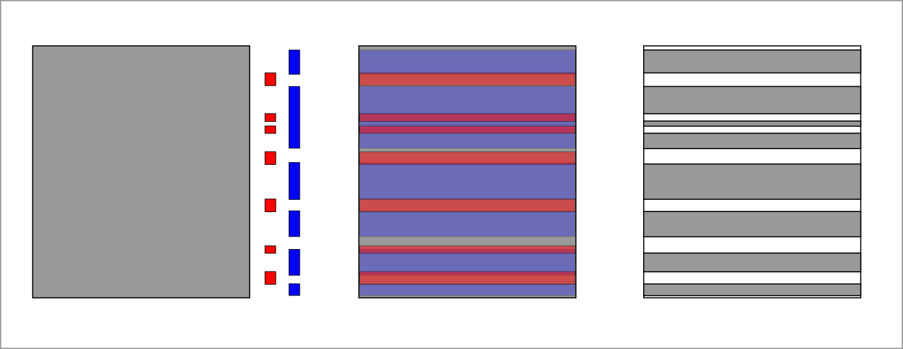
Repeat elements may appear as thousands or even millions of copies in a genome and, by being near identical, cause problems in short-read mapping. In many analyses, the repeat regions are not important and can be simply removed from the data. The information of repeat locations can be considered a negative mask.

An alternative approach is define which regions of the genome can be reliably analysed using the current technology. This was more of an issue when the sequencing reads were shorter (they used to 35 bases or even shorter; now “short” reads are typically 150 bp paired-end reads, i.e. 150 bp + 150 bp). Here, we use an old and a bit conservative approach to define on which regions the reads can be uniquely mapped and generate a positive mask.

Left: A table (grey) and regions of a negative (red) and positive (blue) mask. Middle: Overlay of the masks. Right: The retained parts of the original table (grey).

Repeat masking

The repeat elements have been inferred with the program RepeatMasker (https://www.repeatmasker.org/). The program itself is free and open source, but the repeat libraries (known repeat sequences in different organisms) are not freely available and the analyses are therefore not done on the course. The masking was performed with the command:

$ # RepeatMasker -xsmall -gff -dir ./RM -species "Gasterosteus aculeatus" ninespine.fa

Here, the options -xsmall and -gff specify that the repeat regions are marked in lower-case letters (rather than N’s) in the masked genome and the repeat regions are also outputted as a GFF-file. The known repeat sequences of the three-spined stickleback are used in the search.

We can look at the summery table of masking:

$ less $WORK/shared/reference/RM/ninespine.fa.tbl

The fraction of the genome made of repeat elements is smaller in fish than it is e.g. in humans. (In many plants, a great majority of the genome is made of repeats!) Nevertheless, thousands of repeat elements are found.

The approach used by RepeatMasker is revealed by the raw output file:

$ less $WORK/shared/reference/RM/ninespine.fa.cat.gz

Here, the alignments are BLAST hits between known repeat sequences and regions of the genome. These hits are summarised as table:

$ less $WORK/shared/reference/RM/ninespine.fa.out

but we rather work with a GFF-formatted file. From the RepeatMasker results, we copy the GFF-file and the masked FASTA-file:

$ cp $WORK/shared/reference/RM/ninespine.fa.out.gff reference/ninespine_rm.gff
$ cp $WORK/shared/reference/RM/ninespine.fa.masked reference/ninespine_rm.fa
$ samtools faidx reference/ninespine_rm.fa

The difference between the original and the masked genome file can be visualised with diff:

$ diff reference/ninespine.fa.fai reference/ninespine_rm.fa.fai 
$ diff reference/ninespine.fa reference/ninespine_rm.fa | head -6

84,85c84,85
< TTAGAGACGCTAGCTGGACTTTTCTTGGAGGAATGAATCTTGAGGATGGAGATGATGATG
< ATGATGACAATGAGGCAATGAAGGAAAGAAAGATGTAACTAGAAAATGCATTTCCTGCTG
---
> TTAGAGACGCTAGCTGGACTTTTCTTGGAGGAATGAATCTtgaggatggagatgatgatg
> atgatgacaatgaGGCAATGAAGGAAAGAAAGATGTAACTAGAAAATGCATTTCCTGCTG

The sequences are the same but, in the masked-file, some regions (=inferred repeats) are printed in lower-case characters.

Similarly, the GFF-file looks familiar:

$ head reference/ninespine_rm.gff

##gff-version 2
##date 2016-03-14
##sequence-region ninespine.fa
ctg7180000005484    RepeatMasker    similarity  4961    4993    17.1    +   .   Target "Motif:(TGA)n" 1 33
ctg7180000005484    RepeatMasker    similarity  5395    5448    24.8    +   .   Target "Motif:(GTA)n" 1 53
ctg7180000005484    RepeatMasker    similarity  5577    5870     9.7    -   .   Target "Motif:SINE2-1_GA" 2 314
ctg7180000005484    RepeatMasker    similarity  5944    6056    22.0    +   .   Target "Motif:(TAG)n" 1 110
ctg7180000005484    RepeatMasker    similarity  6248    6340    25.8    +   .   Target "Motif:(TAG)n" 1 94
ctg7180000005484    RepeatMasker    similarity  6528    6636    26.6    +   .   Target "Motif:(TAG)n" 1 109
ctg7180000005484    RepeatMasker    similarity  6733    6757    13.1    +   .   Target "Motif:(G)n" 1 25

The columns of interest are 1, 4 and 5.

We can compress and index them as any other GFF file:

$ bgzip reference/ninespine_rm.gff 
$ tabix reference/ninespine_rm.gff.gz

Positive masking with SNPable

The positive masking is done with Heng Li’s SNPable (https://lh3lh3.users.sourceforge.net/snpable.shtml). The idea of the approach is that the reference genome is split into small fragments and then these fragments are mapped back to the reference. If the fragment can be mapped uniquely, also the corresponding read can be mapped and a variant (=SNP, i.e. single nucleotide polymorphism) within that read region can be identified. Thus the name “SNPable”.

The programs to do the positive mask are available at ‘/projappl/project_2000598/bin/’ (and in the Puhti module “bwa”) but it is not necessary to replicate these steps:


$ splitfa ninespine.fa 75  > frags.fa

$ bwa index ninespine.fa 

$ bwa aln -R 1000000 -O 3 -E 3 ninespine.fa frags.fa > frags.sai
$ bwa samse  ninespine.fa frags.sai frags.fa > frags.sam

$ cat frags.sam | gen_raw_mask.pl > rawMask_75.fa

$ gen_mask -l 75 -r 0.5 rawMask_75.fa > mask_75_50.fa

$ python3 makeMappabilityMask.py 

$ cut -f1 ninespine.fa.fai | while read ctg ; do 
    zcat ninespine_${ctg}.mask.bed.gz | bgzip -c >> ninespine_posmask.bed.gz
  done

$ rm ninespine_[cd]*.mask.bed.gz

Some of the files have been (compressed and) copied to ‘/scratch/project_2000598/shared/reference/snpable/’. A look into the file ‘frags.fa’ reveals that it indeed contains substrings of length 75, starting from the beginning of the reference genome:

$ zcat $WORK/shared/reference/snpable/frags.fa.gz | head

>ctg7180000005484_1
CGTCACACTAACAGCTGCCCATCTGGTTACTGTCAGGGAGAAAACAACTGAGCTTGCGGAGACTTTATGAGGTAC
>ctg7180000005484_2
GTCACACTAACAGCTGCCCATCTGGTTACTGTCAGGGAGAAAACAACTGAGCTTGCGGAGACTTTATGAGGTACT
>ctg7180000005484_3
TCACACTAACAGCTGCCCATCTGGTTACTGTCAGGGAGAAAACAACTGAGCTTGCGGAGACTTTATGAGGTACTG
>ctg7180000005484_4
CACACTAACAGCTGCCCATCTGGTTACTGTCAGGGAGAAAACAACTGAGCTTGCGGAGACTTTATGAGGTACTGG
>ctg7180000005484_5
ACACTAACAGCTGCCCATCTGGTTACTGTCAGGGAGAAAACAACTGAGCTTGCGGAGACTTTATGAGGTACTGGA

( Note that original version from 2009 uses fragments of 35 bases. That was the read length at the time. )

In the next steps those were aligned with bwa aln; this program is outdated and, later on this course, we will use the more advance bwa mem. The final out of SNPable is “FASTA-file” consisting of numbers 0-3, reflecting the uniqueness of the sequence (0=all non-unique; 3=predominantly unique).

$ zcat $WORK/shared/reference/snpable/mask_75_50.fa.gz | head -4

>ctg7180000005484 75 0.500
333333333333333333333333333333333333333333333333333333333333
333333333333333333333333333333333333333333333333333333333333
333333333333333333333333333333333333333333333333333333333333

The final part of the pipeline is Stephan Schiffels’ python script from the msmc-tools package (https://github.com/stschiff/msmc-tools). It generates one BED file (see the format here) per contig and these are then concatenated into one file using a bash loop. We copy that:

$ cp $WORK/shared/reference/snpable/ninespine_posmask.bed.gz reference/
$ tabix reference/ninespine_posmask.bed.gz
$ zcat reference/ninespine_posmask.bed.gz | head -5
ctg7180000005484    0   5046
ctg7180000005484    5117    5404
ctg7180000005484    5670    5924
ctg7180000005484    5992    6103
ctg7180000005484    6210    6287

This file lists the regions that are considered trustworthy. Later on the course, we will use this positive mask to filter our variant data. If you want to create a positive mask for a genome of your own, you may want to check the instructions at http://dx.doi.org/10.1016/j.xpro.2023.102567 on how to parallelise the time consuming steps. However, I think that the 35-bp fragment length used in that study is unnecessary short and makes the mask overly conservative. Even the 75-bp length is pretty short.

Exercise: Repeat annotation and positive masking

The file reference/ninespine_rm.gff.gz contains repeat annotations for the reference genome, reference/ninespine_rm.fa the sequence with repeats indicated in the lower case, and reference/ninespine_posmask.bed.gz annotations of the regions that are considered “mappable” using the SNPable tool. Find some information of them.

Exercise 3 in Moodle.

Another visual view on a reference genome

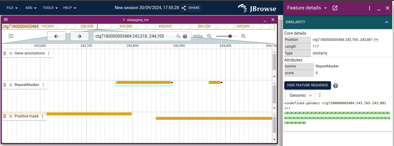
With these resources, we can have another look at the reference genome at https://popgeno.biocenter.helsinki.fi/jbrowse2/. Open up the “Linear Genome View” and then add the tracks “Gene annotations”, “RepeatMasker” and “Positive mask”. If you browse to “ctg7180000005484:243,518..244,105” (or copy that location to the locus field in the middle top), you can see something like this:

I have clicked the RepeatMasker element in the middle and opened up the feature sequence. It reveals that the repeat element is a (CA)n microsatellite, that is the bases “CA” are repeated many times in a row. The positive mask has a gap around that microsat as 75-bp fragments consisting of CAs only cannot be uniquely placed in the reference; if they contain enough flanking sequence, they can be mapped.

Browsing around shows that often (but not always) a gap in the positive mask overlaps with annotated repeat elements. A comparison to gene annotations would show that most coding regions are unique and positively masked.

Own installation of JBrowse2

The JBrowse2 software is freely available to different operating systems at https://jbrowse.org/jb2/.

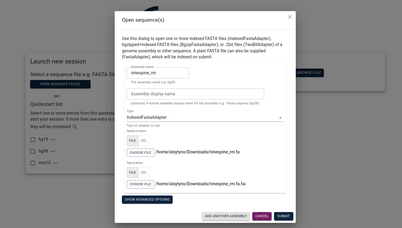
The easiest way to start with a local JBrowse2 is to download the data files to one’s own computer. For this, I have downloaded “ninespine_rm.fa”, “ninespine_rm.fa.fai”, “ninespine_annotation_sorted.gff3.gz” and “ninespine_annotation_sorted.gff3.gz.tbi”. On the start screen, one needs to click “Open sequence files” and then fill at least “Assembly name”, “FastaLocation” and “FaiLocation”.

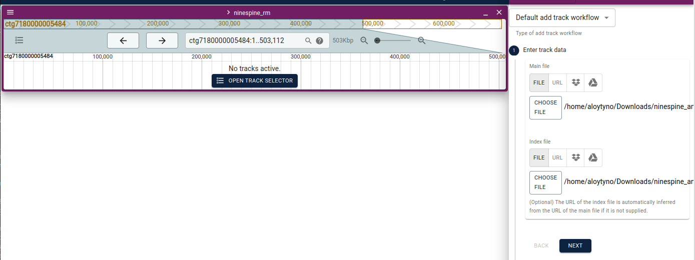
After opening the genome view, one can click “Open track selector” and then yellow plus sign (right bottom corner), choosing “Add track”. Now one has to define the track file and its index, the software can guess its type:

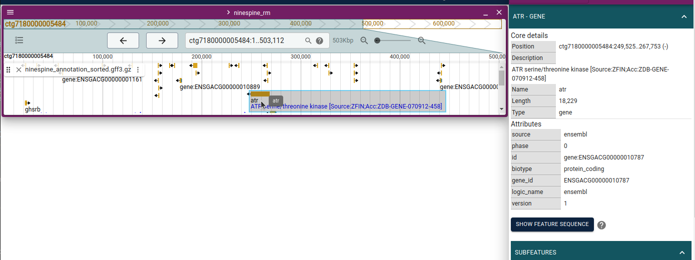
One can change “trackName” to one’s own liking. This now shows the genome and the new track:

Accessing data on Puhti remotely

If the data files are very large or keep changing, downloading them to a local computer can be time consuming. There is a trick to access them remotely, without download, from Puhti.

Computers have “ports” that they use to communicate with different software. Ports with small numbers are reserved for central software, e.g. SSH communicates through port 22. Ports with larger numbers can be used by others; the problem is that these ports are closed to outside world for security reasons.

The trick is to “tunnel” one specific port through SSH and communicate through that between a local computer and a Puhti login node. Only few port numbers between 5,000 and 10,000 are used by specific software and a random number in that range is probably free to be used by a regular user. One should note though that two users on the same computer cannot use the same port for their own communication. Because of that, no specific port number is shown here and below “XXXX” means a number between 5000-9999.

One can open a tunnel from one’s own computer to Puhti with the command:

$ ssh -L XXXX:localhost:XXXX username@puhti.csc.fi

One can then go to the target directory and start a http-server that communicates through the chosen port:

$ cd /scratch/project_2000598/$USER
$ python3 -m http.server XXXX

If one now opens a web browser at the URL “http://localhost:XXXX” (again, “XXXX” is the chosen port number), one should see the contents of that directory. One point to one of the files and (on Linux) right-click with the mouse and select “Copy link address”.

In the JBrowse2 examples above, the FASTA and GFF-files were loaded from the local drive. However, in the menus, there is button “URL” next to “FILE”. If one chooses “URL”, one can paste the URL link saved previously (see “Copy link address” above) and make the program to read the data through the tunnel from Puhti. The same trick works for the genome and the track files.

Note that the Python http-server has to be running all the time. One can close the connection by stopping the http server and logging out from Puhti.

Take-home message

The course works are done on CSC Puhti and require skills learned at EEB-021. Please rehearse the central ommands at https://intscicom.biocenter.helsinki.fi if you feel uncertain about them.

The continuity of the reference genome is not especially important for population genetic studies as long as the genome is largely haploid, i.e. each region is represented only once. In the first practicals, we use a small fraction of the draft assembly of the nine-spined stickleback genome. This draft assembly consists of “contigs”, i.e. continuous fragments of genome sequence produced by the assembly program. These contigs were later connected to each other, known as “scaffolding”, to create nearly continuos chromosome sequences. As these sequences are not complete and shown experimentally to belong together, they are called “linkage groups”, meaning that they appear to be associated.

The reference genome is typically stored in the FASTA format, often compressed to reduce its size. There are various types of meta-data to provide information about specific regions in the genome. Common formats for “region data” are GFF and BED. Confusingly, these formats follow two different specifications, and GFF is “1-start” and “fully-closed” (or “1-based” and “inclusive”) whereas BED is “0-start” and “half-closed”. Any region data can be compressed and indexed, allowing fast retrieval of entries overlapping with a query region.

Reference genomes and their meta-data can be visualised with genome browser programs such JBrowse2. The software runs on all popular computer platforms.